Occasionally I will want to see long-term historical data so I can better interpret the history of something I’m trying to analyze. I wrote some code a while back that analyzes the increased cost of monthly housing payments due to increases in mortgage rates. However, recently I wanted to re-write this code but apply it to the Arizona housing market. The only issue was I was only able to download historical data for Arizona median house sales prices back to 2001. As well I could only download Real Per Capita Personal Income for Arizona back to January 2008. So in these examples below what I’m going to do it use highly correlated datasets with a close enough relationship to my dependent variables to estimate these values back a few decades. The whole purpose of this dataset is to get an idea of home ownership affordability to predict high and low housing prices.

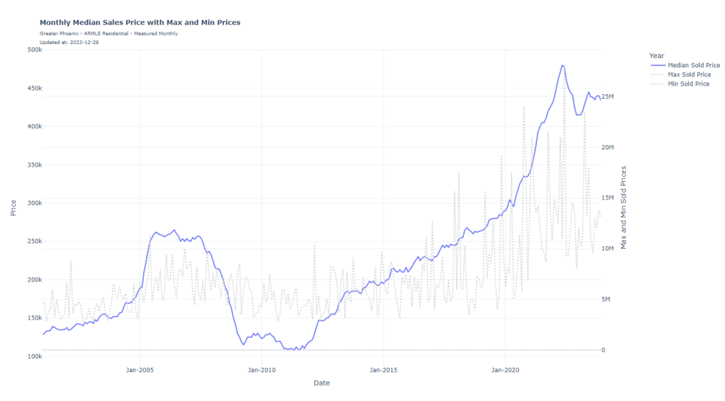
When I looked at the historical median sales price of houses in Arizona I didn’t feel this limited dataset gave quality insight into the high cost of housing relative to high real estate prices combined with high mortgage rates. As shown in the chart below you can see the national payment-to-income ratio going back to 1971. The AZ dataset is too limited.


You can see that house payments relative to income are historically higher than they have ever been by a significant margin. The Arizona dataset shows this but it’s not quite as apparent due to the limited timeframe (only going back to 2001).
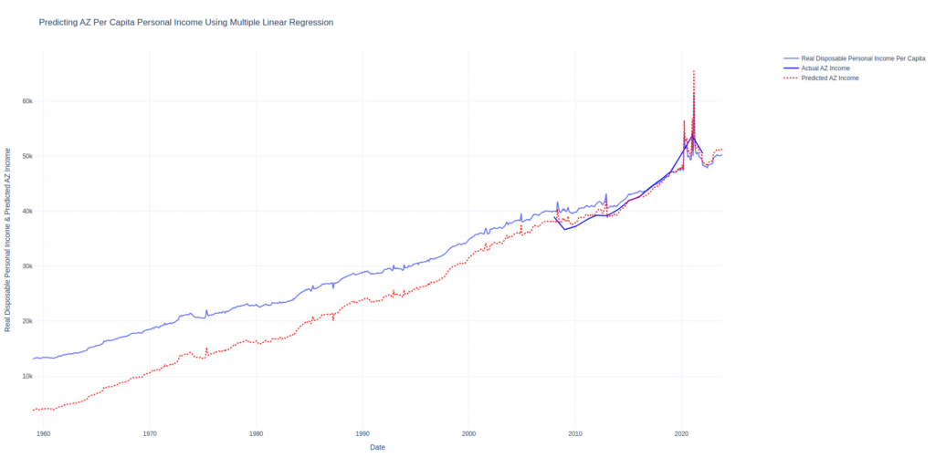
Two datasets are missing historically here we’re going to use multiple linear regression to estimate. To establish the Real Per Capita Income for Arizona I will use just linear regression with one regressor, Real Disposable Personal Income: Per Capita (A229RX0) The reason I’m using this regressor is the data is updated monthly and goes back over 60 years. This means my plots will have large historical data plus they will be up to date rather than being delayed a few years since the data we’re estimating, Real Per Capita Personal Income for Arizona (AZRPIPC), is only updated once per year.

In this chart, our actual data is the solid dark blue line. Our regressor is the solid light blue line and the predicted data is the dotted red line. The MAPE on this data is 3.21%. Keep in mind this should interpreted lightly as this value is on all training data. There is no train/test dataset. I’m just looking for a projection of historical values.
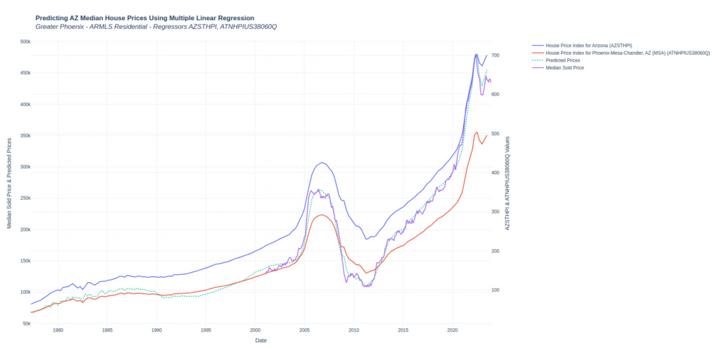
The next dataset that I’m missing historical data for is the median sales price of a house in Arizona. I can pull monthly values from ARMLS back to 2001. So the goal is to use multiple linear regression using All-Transactions House Price Index for Arizona (AZSTHPI) and All-Transactions House Price Index for Phoenix-Mesa-Chandler, AZ (MSA) (ATNHPIUS38060Q) as regressors. The MAPE on this model is 3.21% on training data.

You can see in the chart that I only have the median house prices going back to 2001. My regressors are in blue and red where the predicted historical values of median house prices are in dotted teal.
