At times when creating trading strategies using big data you need access to historical economic data. One of the best sources of data is the Economic Research branch of the St. Louis Federal Reserve or FRED. Today I’m going to show you how to pull that data into a dataframe so that you can analyze it using machine learning or AI.
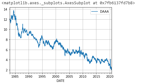
The first step is to import Pandas datareader. What this piece of code does is it downloads all the data for Corporate AAA bond yields. Every dataset in FRED has a symobl. In this case it’s DAAA.
import pandas_datareader.data as web
import datetime

today = pd.to_datetime("today")
start = datetime.datetime(1900, 1, 1)
end = today

df_Corp_AAA_yield = web.DataReader(['DAAA'], 'fred', start, end)

# not working - Corp_AAA_yield = web.DataReader(['DAAA'], 'fred', start, end)
df_Corp_AAA_yield.head()
df_Corp_AAA_yield.tail()
We can now visualize our dataframe by plotting it.
When analyzing historical time frame data in machine learning it needs to be normalized. In this code example, I will show how to get S&P data then convert it to a percent of daily increase/decrease as well as a logarithmic daily increase/decrease.
The first part of this code will use yfinance as our datasource.
#we're going to use yfinance as our data source
!pip install yfinance --upgrade --no-cache-dir

import pandas as pd
import numpy as np
import yfinance as yf
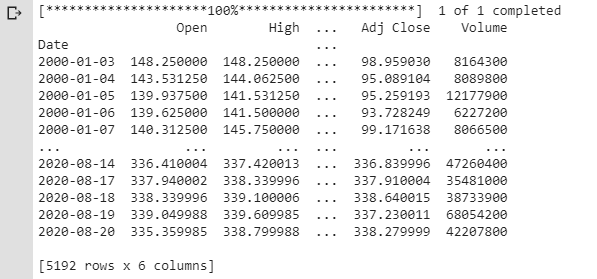
Next, we’re going to create a dataframe called df and download SPY data from 2000 to it.
#Here we're creating a dataframe for spy data from 2000-current
df = yf.download('spy',
  start='2000-01-01',
  end='2020-08-21',
  progress=True)
  #dauto_adjust=True,
  #actions='inline',) #adjust for stock splits and dividends
#print the dataframe to see what lives in it
print(df)
Finally, we’ll print the result of df so you can get an idea of what is inside of it.
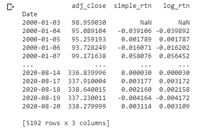
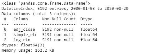
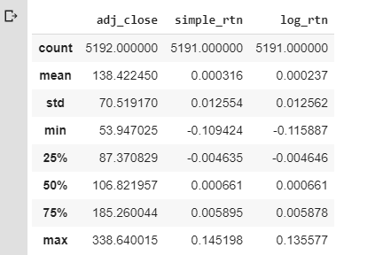
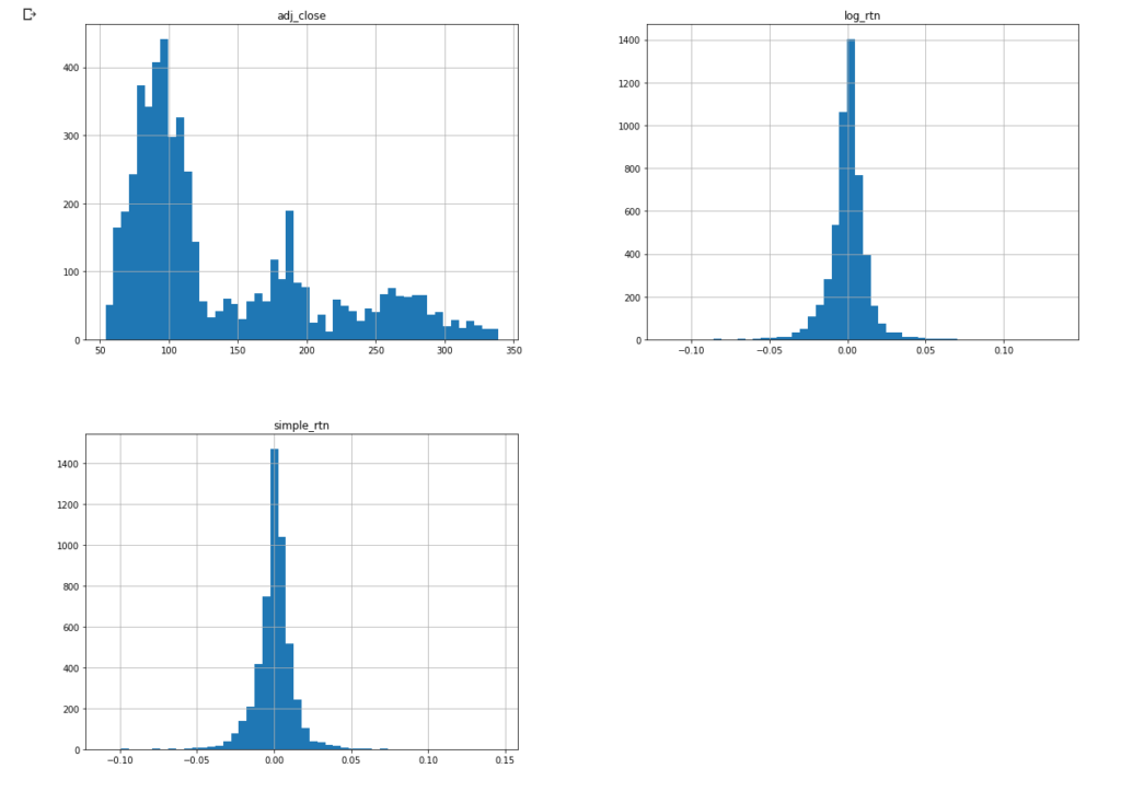
We’re going to drop all the columns except Adj Close. Then we’ll rename it adj_close. Next, we’ll create a column labeled simple_rtn. This is the daily simple return or percent increase/decrease. The next line of code creates a logarithmic increase/decrease. Logarithmic gives equal bearing to the Y-axis and can be defined as follows, “A logarithmic price scale uses the percentage of change to plot data points, so, the scale prices are not positioned equidistantly. A linear price scale uses an equal value between price scales providing an equal distance between values.”
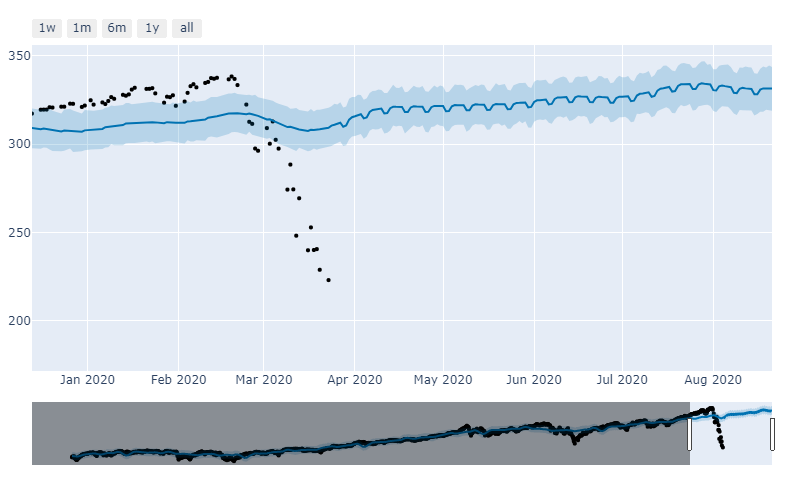
A few years ago Facebook decided to open source Prophet. This is their analytics algorithm that uses an additive model to fit non-linear data with seasonality. I started to wonder, “If this algorithm were in place in March when the stock market’s crashed what would it have advised?” So I decided to give it a spin.
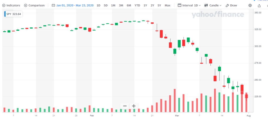
Let’s assume you had a significant amount of money invested in S&P index funds on March 23, 2020. Since the beginning of the year, you would have lost 31% of your money. At this point you might be thinking, “Oh shit, what do I do, sell, buy, hold?”. A lot of investors would panic and sell. The market thrives and two psychologies, fear and greed.
But let’s take an analytics approach to this problem. What would Facebook’s Prophet algorithm advise you do to? Here is how you can approach that problem.
The first thing I did was fire up Google Colab. The entire notebook can be found here.
The first part of this code uses a Python DataReader to pull SPY from Yahoo Finance. I created an end date of 3/23/2020. This only gives Facebook’s Prophet access to data up until this point. We are then going to have it predict where it thinks the price would be today 8/20/2020 without feeding it any future data.
# Python
import pandas as pd
from fbprophet import Prophet

from pandas_datareader import data as web
import datetime

import pandas as pd
import matplotlib.pyplot as plt

stock = 'spy'
endDate = datetime.datetime(2020, 3, 23)
#start_date = (datetime.datetime.now() - datetime.timedelta(days=2000)).strftime("%m-%d-%Y")
start_date = (endDate - datetime.timedelta(days=2000)).strftime("%m-%d-%Y")
#print(start_date)
df = web.DataReader(stock, data_source='yahoo', start=start_date,end=endDate)
#date is the index so you need to make it a column
df["Date"] = df.index

import matplotlib.pyplot as plt

plt.plot(df['Close'])
df.head()
df.tail()
The next part of code renames the imported columns from “Date” to “ds” and “Close” to “y”. DS and Y are the two variables that Prophet will be looking for.
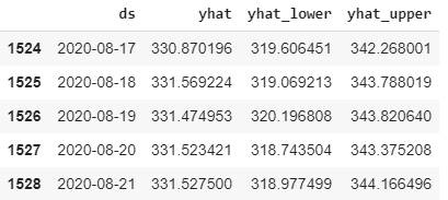
This next part of the code starts to set up Prophet. The only variable you should be concerned with is 151. This is telling the algorithm to look out 151 days. Then it forecasts three variables yhat, yhat_lower, and yhat_upper. Yhat is the predicted price with upper and lower being the bounds in which it assumes the price will fall in.
You can see that it predicts the closing price for tomorrow will be 331.52. Remember it is only using data from March 23rd to make this calculation. Given the wild gyrations in the market, this is extremely close to being accurate. The SPY closed today at 338. Prophet predicted it would close at 331. It was off by 2%. This is using a 5-month look ahead forecasting model.
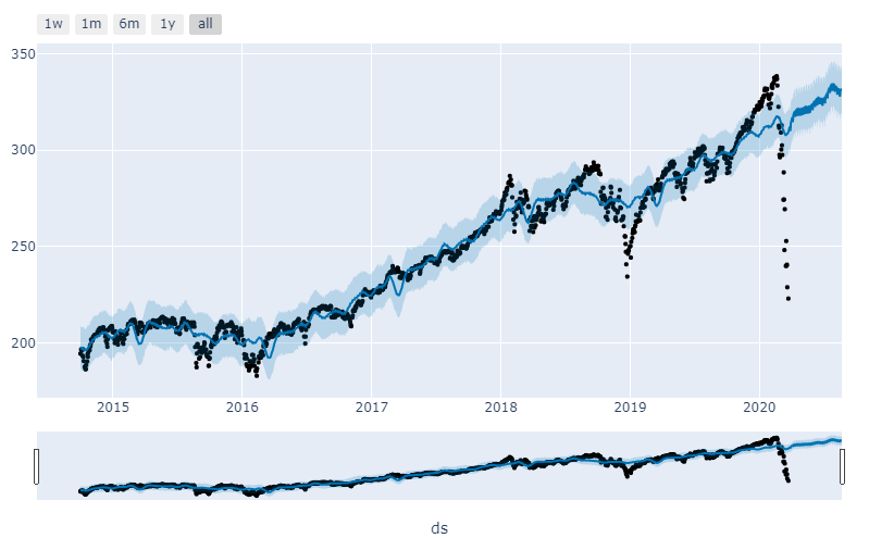
Here is the visual representation of what that looks like.
from fbprophet.plot import plot_plotly, plot_components_plotly

plot_plotly(m, forecast)
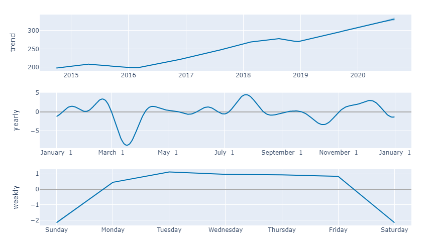
And more charts…
plot_components_plotly(m, forecast)
Finally here is the visualization of the predicted price vs. the actual price chart.