I find myself listening to videos on YouTube quite frequently where it would be nice to dump them into an MP3 and take them on the road. This script will do exactly that. I also added transcription for analysis. Just put in your link and it will generate the MP3 and TXT file.
Polymarket.com, a prediction market platform, operates on the Ethereum blockchain through the Polygon network, making it possible to analyze user transactions directly from the blockchain. By accessing a user’s wallet address, we can examine their trades in detail, track profit/loss, and monitor position changes over time. In this post, I’ll show how you can leverage the Polygon blockchain data to analyze trades on Polymarket using wallet IDs and some helpful Python code.
Below are examples of the kinds of charts the script generates and their significance.
Shares by Market
This chart focuses on the number of shares the user holds across different markets. It’s another way to visualize their exposure to various outcomes but focuses on the number of shares rather than their total purchase value.
Insight: Larger bars suggest higher exposure to specific markets. The average price paid per share is also annotated, providing further context.
Purpose: Useful for understanding the user’s position size in each market.
Total Purchase Value by Market
In this bar chart, the user’s total purchase value is broken down by market. The height of each bar indicates how much the user has invested in each specific market.
Purpose: It allows for a clear visualization of where the user is concentrating their funds, showing which markets hold the largest portion of their portfolio.
Insight: The accompanying labels provide information about the average price paid per share in each market, helping understand whether the user is buying low or high within a market.
Total Purchase Value Timeline
This scatter plot shows the timeline of the user’s trades by plotting the total purchase value of trades over time.
Purpose: This chart reveals when the user made their largest investments, showing the fluctuations in purchase value across trades.
Insight: Each dot represents a trade, with its position on the Y-axis showing the value and on the X-axis showing the timestamp of the transaction. You can use this chart to understand when the user made big moves in the market.
Holdings by Market and Outcome (Treemap)
The treemap provides a more detailed look at the user’s holdings, breaking down their positions by both market and outcome. Each rectangle represents the shares held in a particular market-outcome pair, with the size of the rectangle proportional to the user’s investment.
Purpose: Ideal for visually assessing how much the user has allocated to each market and outcome combination.
Insight: It highlights not just which markets the user has invested in but also how they’ve distributed their bets across different outcomes within those markets.
Holdings Distribution by Market (Pie Chart)
This pie chart visualizes the user’s current holdings, showing the percentage distribution of shares across different markets.
Purpose: Offers a high-level overview of the user’s portfolio diversification across different markets.
Insight: Larger slices indicate heavier investments in specific markets, allowing you to quickly see where the user has concentrated their bets.
Cumulative Shares Over Time
This line chart tracks the cumulative number of shares held by the user in various markets over time. It helps visualize when the user bought or sold shares and how their position has evolved in each market.
Purpose: This chart is essential for understanding the user’s trading strategy over time, revealing periods of heavy buying or selling.
Insight: Each line represents a different market and outcome combination. Peaks in the lines indicate increased positions, while dips show reductions or sales.
The Code
The code behind these charts fetches data from Polygon’s blockchain and processes the transactions associated with a given wallet ID. It retrieves ERC-1155 and ERC-20 token transaction data, enriches it with market information, and generates visual insights based on trading activity. You can use this code to analyze any Polymarket user’s trades simply by knowing their wallet address.
Here’s a breakdown of the main functions:
fetch_user_transactions(wallet_address, api_key): Fetches all ERC-1155 and ERC-20 transactions for a given wallet from Polygon.
add_financial_columns(): Processes transactions to calculate key financial metrics like profit/loss, total purchase value, and shares held.
plot_profit_loss_by_trade(): Generates a bar plot showing profit or loss for each trade.
plot_shares_over_time(): Creates a line plot showing cumulative shares over time.
create_and_save_pie_chart(): Generates a pie chart that breaks down holdings by market.
create_and_save_treemap(): Produces a treemap for holdings based on market and outcome.
plot_total_purchase_value(): Generates a scatter plot showing total purchase value over time.
This tool offers deep insights into any user’s trading behavior and performance on Polymarket.
import os
import requests
import logging
import pandas as pd
import subprocess
import json
import time
from dotenv import load_dotenv
import plotly.express as px
import re
from bs4 import BeautifulSoup
from importlib import reload
import numpy as np
import argparse
import os
import subprocess
import json
import logging
import pandas as pd
from dotenv import load_dotenv
logging.basicConfig(level=logging.DEBUG, format='%(asctime)s - %(levelname)s - %(message)s')
logger = logging.getLogger(__name__)
# Load environment variables
load_dotenv("keys.env")
price_cache = {}
# EXCHANGES
CTF_EXCHANGE = '0x2791Bca1f2de4661ED88A30C99A7a9449Aa84174'
NEG_RISK_CTF_EXCHANGE = '0x4d97dcd97ec945f40cf65f87097ace5ea0476045'
# SPENDERS FOR EXCHANGES
NEG_RISK_CTF_EXCHANGE_SPENDER = '0xC5d563A36AE78145C45a50134d48A1215220f80a'
NEG_RISK_ADAPTER = '0xd91E80cF2E7be2e162c6513ceD06f1dD0dA35296'
CTF_EXCHANGE_SPENDER = '0x4bFb41d5B3570DeFd03C39a9A4D8dE6Bd8B8982E'
CACHE_EXPIRATION_TIME = 60 * 30 # Cache expiration time in seconds (5 minutes)
PRICE_CACHE_FILE = './data/live_price_cache.json'
# Dictionary to cache live prices
live_price_cache = {}
def load_price_cache():
"""Load the live price cache from a JSON file."""
if os.path.exists(PRICE_CACHE_FILE):
try:
with open(PRICE_CACHE_FILE, 'r') as file:
return json.load(file)
except json.JSONDecodeError as e:
logger.error(f"Error loading price cache: {e}")
return {}
return {}
def save_price_cache(cache):
"""Save the live price cache to a JSON file."""
with open(PRICE_CACHE_FILE, 'w') as file:
json.dump(cache, file)
def is_cache_valid(cache_entry, expiration_time=CACHE_EXPIRATION_TIME):
"""
Check if the cache entry is still valid based on the current time and expiration time.
"""
if not cache_entry:
return False
cached_time = cache_entry.get('timestamp', 0)
return (time.time() - cached_time) < expiration_time
def call_get_live_price(token_id, expiration_time=CACHE_EXPIRATION_TIME):
"""
Get live price from cache or update it if expired.
"""
logger.info(f'Getting live price for token {token_id}')
# Load existing cache
price_cache = load_price_cache()
cache_key = f"{token_id}"
# Check if cache is valid
if cache_key in price_cache and is_cache_valid(price_cache[cache_key], expiration_time):
logger.info(f'Returning cached price for {cache_key}')
return price_cache[cache_key]['price']
# If cache is expired or doesn't exist, fetch live price
try:
result = subprocess.run(
['python3', 'get_live_price.py', token_id],
stdout=subprocess.PIPE,
stderr=subprocess.PIPE,
text=True,
check=True
)
# Parse the live price from the subprocess output
output_lines = result.stdout.strip().split("\n")
live_price_line = next((line for line in output_lines if "Live price for token" in line), None)
if live_price_line:
live_price = float(live_price_line.strip().split(":")[-1].strip())
else:
logger.error("Live price not found in subprocess output.")
return None
logger.debug(f"Subprocess get_live_price output: {result.stdout}")
# Update cache with the new price and timestamp
price_cache[cache_key] = {'price': live_price, 'timestamp': time.time()}
save_price_cache(price_cache)
return live_price
except subprocess.CalledProcessError as e:
logger.error(f"Subprocess get_live_price error: {e.stderr}")
return None
except Exception as e:
logger.error(f"Error fetching live price: {str(e)}")
return None
def update_live_price_and_pl(merged_df, contract_token_id, market_slug=None, outcome=None):
"""
Calculate the live price and profit/loss (pl) for each trade in the DataFrame.
"""
# Ensure tokenID in merged_df is string
merged_df['tokenID'] = merged_df['tokenID'].astype(str)
contract_token_id = str(contract_token_id)
# Check for NaN or empty token IDs
if not contract_token_id or contract_token_id == 'nan':
logger.warning("Encountered NaN or empty contract_token_id. Skipping.")
return merged_df
# Add live_price and pl columns if they don't exist
if 'live_price' not in merged_df.columns:
merged_df['live_price'] = np.nan
if 'pl' not in merged_df.columns:
merged_df['pl'] = np.nan
# Filter rows with the same contract_token_id and outcome
merged_df['outcome'] = merged_df['outcome'].astype(str)
matching_rows = merged_df[(merged_df['tokenID'] == contract_token_id) &
(merged_df['outcome'].str.lower() == outcome.lower())]
if not matching_rows.empty:
logger.info(f'Fetching live price for token {contract_token_id}')
live_price = call_get_live_price(contract_token_id)
logger.info(f'Live price for token {contract_token_id}: {live_price}')
if live_price is not None:
try:
# Calculate profit/loss based on the live price
price_paid_per_token = matching_rows['price_paid_per_token']
total_purchase_value = matching_rows['total_purchase_value']
pl = ((live_price - price_paid_per_token) / price_paid_per_token) * total_purchase_value
# Update the DataFrame with live price and pl
merged_df.loc[matching_rows.index, 'live_price'] = live_price
merged_df.loc[matching_rows.index, 'pl'] = pl
except Exception as e:
logger.error(f"Error calculating live price and profit/loss: {e}")
else:
logger.warning(f"Live price not found for tokenID {contract_token_id}")
merged_df.loc[matching_rows.index, 'pl'] = np.nan
return merged_df
def find_token_id(market_slug, outcome, market_lookup):
"""Find the token_id based on market_slug and outcome."""
for market in market_lookup.values():
if market['market_slug'] == market_slug:
for token in market['tokens']:
if token['outcome'].lower() == outcome.lower():
return token['token_id']
return None
def fetch_data(url):
"""Fetch data from a given URL and return the JSON response."""
try:
response = requests.get(url, timeout=10) # You can specify a timeout
response.raise_for_status() # Raise an error for bad responses (4xx, 5xx)
return response.json()
except requests.exceptions.RequestException as e:
logger.error(f"Error fetching data from URL: {url}. Exception: {e}")
return None
def fetch_all_pages(api_key, token_ids, market_slug_outcome_map, csv_output_dir='./data/polymarket_trades/'):
page = 1
offset = 100
retry_attempts = 0
all_data = [] # Store all data here
while True:
url = f"https://api.polygonscan.com/api?module=account&action=token1155tx&contractaddress={NEG_RISK_CTF_EXCHANGE}&page={page}&offset={offset}&startblock=0&endblock=99999999&sort=desc&apikey={api_key}"
logger.info(f"Fetching transaction data for tokens {token_ids}, page: {page}")
data = fetch_data(url)
if data and data['status'] == '1':
df = pd.DataFrame(data['result'])
if df.empty:
logger.info("No more transactions found, ending pagination.")
break # Exit if there are no more transactions
all_data.append(df)
page += 1 # Go to the next page
else:
logger.error(f"API response error or no data found for page {page}")
if retry_attempts < 5:
retry_attempts += 1
time.sleep(retry_attempts)
else:
break
if all_data:
final_df = pd.concat(all_data, ignore_index=True) # Combine all pages
logger.info(f"Fetched {len(final_df)} transactions across all pages.")
return final_df
return None
def validate_market_lookup(token_ids, market_lookup):
valid_token_ids = []
invalid_token_ids = []
for token_id in token_ids:
market_slug, outcome = find_market_info(token_id, market_lookup)
if market_slug and outcome:
valid_token_ids.append(token_id)
else:
invalid_token_ids.append(token_id)
logger.info(f"Valid token IDs: {valid_token_ids}")
if invalid_token_ids:
logger.warning(f"Invalid or missing market info for token IDs: {invalid_token_ids}")
return valid_token_ids
def sanitize_filename(filename):
"""
Sanitize the filename by removing or replacing invalid characters.
"""
# Replace invalid characters with an underscore
return re.sub(r'[\\/*?:"<>|]', '_', filename)
def sanitize_directory(directory):
"""
Sanitize the directory name by removing or replacing invalid characters.
"""
# Replace invalid characters with an underscore
return re.sub(r'[\\/*?:"<>|]', '_', directory)
def extract_wallet_ids(leaderboard_url):
"""Scrape the Polymarket leaderboard to extract wallet IDs."""
logging.info(f"Fetching leaderboard page: {leaderboard_url}")
response = requests.get(leaderboard_url)
if response.status_code != 200:
logging.error(f"Failed to load page {leaderboard_url}, status code: {response.status_code}")
return []
logging.debug(f"Page loaded successfully, status code: {response.status_code}")
soup = BeautifulSoup(response.content, 'html.parser')
logging.debug("Page content parsed with BeautifulSoup")
wallet_ids = []
# Debug: Check if <a> tags are being found correctly
a_tags = soup.find_all('a', href=True)
logging.debug(f"Found {len(a_tags)} <a> tags in the page.")
for a_tag in a_tags:
href = a_tag['href']
logging.debug(f"Processing href: {href}")
if href.startswith('/profile/'):
wallet_id = href.split('/')[-1]
wallet_ids.append(wallet_id)
logging.info(f"Extracted wallet ID: {wallet_id}")
else:
logging.debug(f"Skipped href: {href}")
return wallet_ids
def load_market_lookup(json_path):
"""Load market lookup data from a JSON file."""
with open(json_path, 'r') as json_file:
return json.load(json_file)
def find_market_info(token_id, market_lookup):
"""Find market_slug and outcome based on tokenID."""
token_id = str(token_id) # Ensure token_id is a string
if not token_id or token_id == 'nan':
logger.warning("Token ID is NaN or empty. Skipping lookup.")
return None, None
logger.debug(f"Looking up market info for tokenID: {token_id}")
for market in market_lookup.values():
for token in market['tokens']:
if str(token['token_id']) == token_id:
logger.debug(
f"Found market info for tokenID {token_id}: market_slug = {market['market_slug']}, outcome = {token['outcome']}")
return market['market_slug'], token['outcome']
logger.warning(f"No market info found for tokenID: {token_id}")
return None, None
def fetch_data(url):
"""Fetch data from a given URL and return the JSON response."""
response = requests.get(url)
return response.json()
def save_to_csv(filename, data, headers, output_dir):
"""Save data to a CSV file in the specified output directory."""
filepath = os.path.join(output_dir, filename)
with open(filepath, 'w', newline='') as file:
writer = csv.DictWriter(file, fieldnames=headers)
writer.writeheader()
for entry in data:
writer.writerow(entry)
logger.info(f"Saved data to {filepath}")
def add_timestamps(erc1155_df, erc20_df):
"""
Rename timestamp columns and convert them from UNIX to datetime.
"""
# Rename the timestamp columns to avoid conflicts during merge
erc1155_df.rename(columns={'timeStamp': 'timeStamp_erc1155'}, inplace=True)
erc20_df.rename(columns={'timeStamp': 'timeStamp_erc20'}, inplace=True)
# Convert UNIX timestamps to datetime format
erc1155_df['timeStamp_erc1155'] = pd.to_numeric(erc1155_df['timeStamp_erc1155'], errors='coerce')
erc20_df['timeStamp_erc20'] = pd.to_numeric(erc20_df['timeStamp_erc20'], errors='coerce')
erc1155_df['timeStamp_erc1155'] = pd.to_datetime(erc1155_df['timeStamp_erc1155'], unit='s', errors='coerce')
erc20_df['timeStamp_erc20'] = pd.to_datetime(erc20_df['timeStamp_erc20'], unit='s', errors='coerce')
return erc1155_df, erc20_df
def enrich_erc1155_data(erc1155_df, market_lookup):
"""
Enrich the ERC-1155 DataFrame with market_slug and outcome based on market lookup.
"""
def get_market_info(token_id):
if pd.isna(token_id) or str(token_id) == 'nan':
return 'Unknown', 'Unknown'
for market in market_lookup.values():
for token in market['tokens']:
if str(token['token_id']) == str(token_id):
return market['market_slug'], token['outcome']
return 'Unknown', 'Unknown'
erc1155_df['market_slug'], erc1155_df['outcome'] = zip(
*erc1155_df['tokenID'].apply(lambda x: get_market_info(x))
)
return erc1155_df
def get_transaction_details_by_hash(transaction_hash, api_key, output_dir='./data/polymarket_trades/'):
"""
Fetch the transaction details by hash from Polygonscan, parse the logs, and save the flattened data as a CSV.
Args:
- transaction_hash (str): The hash of the transaction.
- api_key (str): The Polygonscan API key.
- output_dir (str): The directory to save the CSV file.
Returns:
- None: Saves the transaction details to a CSV.
"""
# Ensure output directory exists
os.makedirs(output_dir, exist_ok=True)
# Construct the API URL for fetching transaction receipt details by hash
url = f"https://api.polygonscan.com/api?module=proxy&action=eth_getTransactionReceipt&txhash={transaction_hash}&apikey={api_key}"
logger.info(f"Fetching transaction details for hash: {transaction_hash}")
logger.debug(f"Request URL: {url}")
try:
# Fetch transaction details
response = requests.get(url)
logger.debug(f"Polygonscan API response status: {response.status_code}")
if response.status_code != 200:
logger.error(f"Non-200 status code received: {response.status_code}")
return None
# Parse the JSON response
data = response.json()
logger.debug(f"Response JSON: {data}")
# Check if the status is successful
if data.get('result') is None:
logger.error(f"Error in API response: {data.get('message', 'Unknown error')}")
return None
# Extract the logs
logs = data['result']['logs']
logs_df = pd.json_normalize(logs)
# Save the logs to a CSV file for easier review
csv_filename = os.path.join(output_dir, f"transaction_logs_{transaction_hash}.csv")
logs_df.to_csv(csv_filename, index=False)
logger.info(f"Parsed logs saved to {csv_filename}")
return logs_df
except Exception as e:
logger.error(f"Exception occurred while fetching transaction details for hash {transaction_hash}: {e}")
return None
def add_financial_columns(erc1155_df, erc20_df, wallet_id, market_lookup):
"""
Merge the ERC-1155 and ERC-20 dataframes, calculate financial columns,
including whether a trade was won or lost, and fetch the latest price for each contract and tokenID.
"""
# Merge the two dataframes on the 'hash' column
merged_df = pd.merge(erc1155_df, erc20_df, how='outer', on='hash', suffixes=('_erc1155', '_erc20'))
# Convert wallet ID and columns to lowercase for case-insensitive comparison
wallet_id = wallet_id.lower()
merged_df['to_erc1155'] = merged_df['to_erc1155'].astype(str).str.lower()
merged_df['from_erc1155'] = merged_df['from_erc1155'].astype(str).str.lower()
# Remove rows where 'tokenID' is NaN or 'nan'
merged_df['tokenID'] = merged_df['tokenID'].astype(str)
merged_df = merged_df[~merged_df['tokenID'].isnull() & (merged_df['tokenID'] != 'nan')]
# Set transaction type based on wallet address
merged_df['transaction_type'] = 'other'
merged_df.loc[merged_df['to_erc1155'] == wallet_id, 'transaction_type'] = 'buy'
merged_df.loc[merged_df['from_erc1155'] == wallet_id, 'transaction_type'] = 'sell'
# Calculate the purchase price per token and total dollar value
if 'value' in merged_df.columns and 'tokenValue' in merged_df.columns:
merged_df['price_paid_per_token'] = merged_df['value'].astype(float) / merged_df['tokenValue'].astype(float)
merged_df['total_purchase_value'] = merged_df['value'].astype(float) / 10**6 # USDC has 6 decimal places
merged_df['shares'] = merged_df['total_purchase_value'] / merged_df['price_paid_per_token']
else:
logger.error("The necessary columns for calculating purchase price are missing.")
return merged_df
# Create the 'lost' and 'won' columns
merged_df['lost'] = (
(merged_df['to_erc1155'] == '0x0000000000000000000000000000000000000000') &
(merged_df['transaction_type'] == 'sell') &
(merged_df['price_paid_per_token'].isna() | (merged_df['price_paid_per_token'] == 0))
).astype(int)
merged_df['won'] = (
(merged_df['transaction_type'] == 'sell') &
(merged_df['price_paid_per_token'] == 1)
).astype(int)
merged_df.loc[merged_df['lost'] == 1, 'shares'] = 0
merged_df.loc[merged_df['lost'] == 1, 'total_purchase_value'] = 0
# Fetch live prices and calculate profit/loss (pl)
merged_df['tokenID'] = merged_df['tokenID'].astype(str)
merged_df = update_latest_prices(merged_df, market_lookup)
return merged_df
def plot_profit_loss_by_trade(df, user_info):
"""
Create a bar plot to visualize aggregated Profit/Loss (PL) by trade, with values rounded to two decimal places and formatted as currency.
Args:
df (DataFrame): DataFrame containing trade data, including 'market_slug', 'outcome', and 'pl'.
user_info (dict): Dictionary containing user information, such as username, wallet address, and other relevant details.
"""
if 'pl' not in df.columns or df['pl'].isnull().all():
logger.warning("No PL data available for plotting. Skipping plot.")
return
username = user_info.get("username", "Unknown User")
wallet_id = user_info.get("wallet_address", "N/A")
positions_value = user_info.get("positions_value", "N/A")
profit_loss = user_info.get("profit_loss", "N/A")
volume_traded = user_info.get("volume_traded", "N/A")
markets_traded = user_info.get("markets_traded", "N/A")
# Combine market_slug and outcome to create a trade identifier
df['trade'] = df['market_slug'] + ' (' + df['outcome'] + ')'
# Aggregate the Profit/Loss (pl) for each unique trade
aggregated_df = df.groupby('trade', as_index=False).agg({'pl': 'sum'})
# Round PL values to two decimal places
aggregated_df['pl'] = aggregated_df['pl'].round(2)
# Format the PL values with a dollar sign for display
aggregated_df['pl_display'] = aggregated_df['pl'].apply(lambda x: f"${x:,.2f}")
# Define a color mapping based on Profit/Loss sign
aggregated_df['color'] = aggregated_df['pl'].apply(lambda x: 'green' if x >= 0 else 'red')
# Create the plot without using the color axis
fig = px.bar(
aggregated_df,
x='trade',
y='pl',
title='',
labels={'pl': 'Profit/Loss ($)', 'trade': 'Trade (Market Slug / Outcome)'},
text='pl_display',
color='color', # Use the color column
color_discrete_map={'green': 'green', 'red': 'red'},
)
# Remove the legend if you don't want it
fig.update_layout(showlegend=False)
# Rotate x-axis labels for better readability and set the main title
fig.update_layout(
title={
'text': 'Aggregated Profit/Loss by Trade',
'y': 0.95,
'x': 0.5,
'xanchor': 'center',
'yanchor': 'top',
'font': {'size': 24}
},
xaxis_tickangle=-45,
margin=dict(t=150, l=50, r=50, b=100)
)
# Prepare the subtitle text with user information
subtitle_text = (
f"Username: {username} | Positions Value: {positions_value} | "
f"Profit/Loss: {profit_loss} | Volume Traded: {volume_traded} | "
f"Markets Traded: {markets_traded} | Wallet ID: {wallet_id}"
)
# Add the subtitle as an annotation
fig.add_annotation(
text=subtitle_text,
xref="paper",
yref="paper",
x=0.5,
y=1.02,
xanchor='center',
yanchor='top',
showarrow=False,
font=dict(size=14)
)
# Save the plot
plot_dir = "./plots/user_trades"
os.makedirs(plot_dir, exist_ok=True)
sanitized_username = sanitize_filename(username)
plot_file = os.path.join(plot_dir, f"{sanitized_username}_aggregated_profit_loss_by_trade.html")
fig.write_html(plot_file)
logger.info(f"Aggregated Profit/Loss by trade plot saved to {plot_file}")
def plot_shares_over_time(df, user_info):
"""
Create a line plot to visualize the cumulative number of shares for each token over time.
Buy orders add to the position, and sell orders subtract from it.
Args:
df (DataFrame): DataFrame containing trade data, including 'timeStamp_erc1155', 'shares', 'market_slug', 'outcome', and 'transaction_type' ('buy' or 'sell').
user_info (dict): Dictionary containing user information, such as username, wallet address, and other relevant details.
"""
if 'shares' not in df.columns or df['shares'].isnull().all():
logger.warning("No 'shares' data available for plotting. Skipping plot.")
return
username = user_info.get("username", "Unknown User")
# Ensure 'timeStamp_erc1155' is a datetime type, just in case it needs to be converted
if df['timeStamp_erc1155'].dtype != 'datetime64[ns]':
df['timeStamp_erc1155'] = pd.to_datetime(df['timeStamp_erc1155'], errors='coerce')
# Drop rows with NaN values in 'timeStamp_erc1155', 'shares', 'market_slug', 'outcome', or 'transaction_type'
df = df.dropna(subset=['timeStamp_erc1155', 'shares', 'market_slug', 'outcome', 'transaction_type'])
# Sort the dataframe by time to ensure the line chart shows the data in chronological order
df = df.sort_values(by='timeStamp_erc1155')
# Combine 'market_slug' and 'outcome' to create a unique label for each token
df['token_label'] = df['market_slug'] + " - " + df['outcome']
# Create a column for 'position_change' which adds shares for buys and subtracts shares for sells based on 'transaction_type'
df['position_change'] = df.apply(lambda row: row['shares'] if row['transaction_type'] == 'buy' else -row['shares'], axis=1)
# Group by 'token_label' and calculate the cumulative position
df['cumulative_position'] = df.groupby('token_label')['position_change'].cumsum()
# Forward fill the cumulative position to maintain it between trades
df['cumulative_position'] = df.groupby('token_label')['cumulative_position'].ffill()
# Create the line plot, grouping by 'token_label' for separate lines per token ID
fig = px.line(
df,
x='timeStamp_erc1155',
y='cumulative_position',
color='token_label', # This ensures each token ID (market_slug + outcome) gets its own line
title=f'Cumulative Shares Over Time for {username}',
labels={'timeStamp_erc1155': 'Trade Time', 'cumulative_position': 'Cumulative Position', 'token_label': 'Token (Market Slug - Outcome)'},
line_shape='linear'
)
# Update layout for better aesthetics
fig.update_layout(
title={
'text': f"Cumulative Number of Shares Over Time for {username}",
'y': 0.95,
'x': 0.5,
'xanchor': 'center',
'yanchor': 'top',
'font': {'size': 20}
},
margin=dict(t=60),
xaxis_title="Trade Time",
yaxis_title="Cumulative Number of Shares",
legend_title="Token (Market Slug - Outcome)"
)
# Save the plot
plot_dir = "./plots/user_trades"
os.makedirs(plot_dir, exist_ok=True)
sanitized_username = sanitize_filename(username)
plot_file = os.path.join(plot_dir, f"{sanitized_username}_shares_over_time.html")
fig.write_html(plot_file)
logger.info(f"Cumulative shares over time plot saved to {plot_file}")
def plot_user_trades(df, user_info):
"""Plot user trades and save plots, adjusting for trades that were lost."""
username = user_info["username"]
wallet_id = user_info["wallet_address"]
# Sanitize only the filename, not the directory
sanitized_username = sanitize_filename(username)
info_text = (
f"Username: {username} | Positions Value: {user_info['positions_value']} | "
f"Profit/Loss: {user_info['profit_loss']} | Volume Traded: {user_info['volume_traded']} | "
f"Markets Traded: {user_info['markets_traded']} | Wallet ID: {wallet_id}"
)
# Ensure the directory exists
os.makedirs("./plots/user_trades", exist_ok=True)
plot_dir = "./plots/user_trades"
# Flag loss trades where to_erc1155 is zero address, transaction_type is sell, and price_paid_per_token is NaN
df['is_loss'] = df.apply(
lambda row: (row['to_erc1155'] == '0x0000000000000000000000000000000000000000')
and (row['transaction_type'] == 'sell')
and pd.isna(row['price_paid_per_token']), axis=1)
# Set shares and total purchase value to zero for loss trades
df.loc[df['is_loss'], 'shares'] = 0
df.loc[df['is_loss'], 'total_purchase_value'] = 0
### Modify for Total Purchase Value by Market (Current holdings)
df['total_purchase_value_adjusted'] = df.apply(
lambda row: row['total_purchase_value'] if row['transaction_type'] == 'buy' else -row['total_purchase_value'],
axis=1
)
grouped_df_value = df.groupby(['market_slug']).agg({
'total_purchase_value_adjusted': 'sum',
'shares': 'sum',
}).reset_index()
# Calculate the weighted average price_paid_per_token
grouped_df_value['weighted_price_paid_per_token'] = (
grouped_df_value['total_purchase_value_adjusted'] / grouped_df_value['shares']
)
# Sort by total_purchase_value in descending order (ignoring outcome)
grouped_df_value = grouped_df_value.sort_values(by='total_purchase_value_adjusted', ascending=False)
# Format the label for the bars (removing outcome)
grouped_df_value['bar_label'] = (
"Avg Price: $" + grouped_df_value['weighted_price_paid_per_token'].round(2).astype(str)
)
fig = px.bar(
grouped_df_value,
x='market_slug',
y='total_purchase_value_adjusted',
barmode='group',
title=f"Current Total Purchase Value by Market for {username}",
labels={'total_purchase_value_adjusted': 'Current Total Purchase Value', 'market_slug': 'Market'},
text=grouped_df_value['bar_label'],
hover_data={'weighted_price_paid_per_token': ':.2f'},
)
fig.update_layout(
title={
'text': f"Current Total Purchase Value by Market for {username}",
'y': 0.95,
'x': 0.5,
'xanchor': 'center',
'yanchor': 'top',
'font': {'size': 20}
},
margin=dict(t=60),
showlegend=False # Remove the legend as you requested
)
fig.add_annotation(
text=info_text,
xref="paper", yref="paper", showarrow=False, x=0.5, y=1.05, font=dict(size=12)
)
# Save the bar plot as an HTML file
plot_file = os.path.join(plot_dir, f"{sanitized_username}_current_market_purchase_value.html")
fig.write_html(plot_file)
logger.info(f"Current market purchase value plot saved to {plot_file}")
### Modify for Trade Quantity by Market (Current holdings)
df['shares_adjusted'] = df.apply(
lambda row: row['shares'] if row['transaction_type'] == 'buy' else -row['shares'], axis=1)
grouped_df_quantity = df.groupby(['market_slug']).agg({
'shares_adjusted': 'sum',
'total_purchase_value': 'sum',
}).reset_index()
# Calculate the weighted average price_paid_per_token
grouped_df_quantity['weighted_price_paid_per_token'] = (
grouped_df_quantity['total_purchase_value'] / grouped_df_quantity['shares_adjusted']
)
grouped_df_quantity = grouped_df_quantity.sort_values(by='shares_adjusted', ascending=False)
grouped_df_quantity['bar_label'] = (
"Quantity: " + grouped_df_quantity['shares_adjusted'].round().astype(int).astype(str) + "<br>" +
"Avg Price: $" + grouped_df_quantity['weighted_price_paid_per_token'].round(2).astype(str)
)
fig = px.bar(
grouped_df_quantity,
x='market_slug',
y='shares_adjusted',
barmode='group',
title=f"Current Trade Quantity by Market for {username}",
labels={'shares_adjusted': 'Current Trade Quantity', 'market_slug': 'Market'},
text=grouped_df_quantity['bar_label'],
)
fig.update_layout(
title={
'text': f"Current Trade Quantity by Market for {username}",
'y': 0.95,
'x': 0.5,
'xanchor': 'center',
'yanchor': 'top',
'font': {'size': 20}
},
margin=dict(t=60),
showlegend=False # Remove the legend as you requested
)
fig.add_annotation(
text=info_text,
xref="paper", yref="paper", showarrow=False, x=0.5, y=1.05, font=dict(size=12)
)
# Save the trade quantity plot as an HTML file
plot_file = os.path.join(plot_dir, f"{sanitized_username}_current_market_trade_quantity.html")
fig.write_html(plot_file)
logger.info(f"Current market trade quantity plot saved to {plot_file}")
### Modify for Total Purchase Value Timeline
df['total_purchase_value_timeline_adjusted'] = df.apply(
lambda row: row['total_purchase_value'] if row['transaction_type'] == 'buy' else -row['total_purchase_value'],
axis=1
)
# Combine 'market_slug' and 'outcome' into a unique label
df['market_outcome_label'] = df['market_slug'] + ' (' + df['outcome'] + ')'
# Create the scatter plot, now coloring by 'market_outcome_label'
fig = px.scatter(
df,
x='timeStamp_erc1155',
y='total_purchase_value_timeline_adjusted',
color='market_outcome_label', # Use the combined label for market and outcome
title=f"Total Purchase Value Timeline for {username}",
labels={
'total_purchase_value_timeline_adjusted': 'Total Purchase Value',
'timeStamp_erc1155': 'Transaction Time',
'market_outcome_label': 'Market/Outcome'
},
hover_data=['market_slug', 'price_paid_per_token', 'outcome', 'hash'],
)
fig.update_layout(
title={
'text': f"Total Purchase Value Timeline for {username}",
'y': 0.95,
'x': 0.5,
'xanchor': 'center',
'yanchor': 'top',
'font': {'size': 20}
},
margin=dict(t=60)
)
fig.add_annotation(
text=info_text,
xref="paper", yref="paper", showarrow=False, x=0.5, y=1.05, font=dict(size=12)
)
# Save the updated plot
plot_file = os.path.join(plot_dir, f"{sanitized_username}_total_purchase_value_timeline_adjusted.html")
fig.write_html(plot_file)
logger.info(f"Total purchase value timeline plot saved to {plot_file}")
def plot_total_purchase_value(df, user_info):
"""Create and save a scatter plot for total purchase value, accounting for buy and sell transactions."""
# Ensure the directory exists
os.makedirs("./plots/user_trades", exist_ok=True)
plot_dir = "./plots/user_trades"
username = user_info["username"]
wallet_id = user_info["wallet_address"]
# Sanitize only the filename, not the directory
sanitized_username = sanitize_filename(username)
info_text = (
f"Username: {username} | Positions Value: {user_info['positions_value']} | "
f"Profit/Loss: {user_info['profit_loss']} | Volume Traded: {user_info['volume_traded']} | "
f"Markets Traded: {user_info['markets_traded']} | Wallet ID: {wallet_id}"
)
# Flag loss trades where to_erc1155 is zero address, transaction_type is sell, and price_paid_per_token is NaN
df['is_loss'] = df.apply(
lambda row: (row['to_erc1155'] == '0x0000000000000000000000000000000000000000')
and (row['transaction_type'] == 'sell')
and pd.isna(row['price_paid_per_token']), axis=1)
# Set shares and total purchase value to zero for loss trades
df.loc[df['is_loss'], 'shares'] = 0
df.loc[df['is_loss'], 'total_purchase_value'] = 0
# Adjust the total purchase value based on the transaction type
df['total_purchase_value_adjusted'] = df.apply(
lambda row: row['total_purchase_value'] if row['transaction_type'] == 'buy' else -row['total_purchase_value'],
axis=1
)
# Create the scatter plot for total purchase value over time
fig = px.scatter(
df,
x='timeStamp_erc1155', # Assuming this is the correct timestamp field
y='total_purchase_value_adjusted', # Adjusted values for buys and sells
color='market_slug', # Use market_slug with outcome as the color
title=f"Current Purchase Value Timeline for {username}", # Update title to reflect "current"
labels={'total_purchase_value_adjusted': 'Adjusted Purchase Value ($)', 'timeStamp_erc1155': 'Transaction Time'},
hover_data=['market_slug', 'price_paid_per_token', 'outcome', 'hash'],
)
# Adjust title positioning and font size
fig.update_layout(
title={
'text': f"Current Purchase Value Timeline for {username}", # Update to "Current"
'y': 0.95,
'x': 0.5,
'xanchor': 'center',
'yanchor': 'top',
'font': {'size': 20}
},
margin=dict(t=60)
)
fig.add_annotation(
text=info_text,
xref="paper", yref="paper", showarrow=False, x=0.5, y=1.05, font=dict(size=12)
)
# Save the scatter plot as an HTML file
plot_file = os.path.join(plot_dir, f"{sanitized_username}_current_purchase_value_timeline.html")
fig.write_html(plot_file)
logger.info(f"Current purchase value timeline plot saved to {plot_file}")
def create_and_save_pie_chart(df, user_info):
"""Create and save a pie chart for user's current holdings."""
# Ensure the directory exists
os.makedirs("./plots/user_trades", exist_ok=True)
plot_dir = "./plots/user_trades"
username = user_info["username"]
wallet_id = user_info["wallet_address"]
sanitized_username = sanitize_filename(username)
info_text = (
f"Username: {username} | Positions Value: {user_info['positions_value']} | "
f"Profit/Loss: {user_info['profit_loss']} | Volume Traded: {user_info['volume_traded']} | "
f"Markets Traded: {user_info['markets_traded']} | Wallet ID: {wallet_id}"
)
# Flag loss trades where to_erc1155 is zero address, transaction_type is sell, and price_paid_per_token is NaN
df['is_loss'] = df.apply(
lambda row: (row['to_erc1155'] == '0x0000000000000000000000000000000000000000')
and (row['transaction_type'] == 'sell')
and pd.isna(row['price_paid_per_token']), axis=1)
# Set shares and total purchase value to zero for loss trades
df.loc[df['is_loss'], 'shares'] = 0
df['shares_adjusted'] = df.apply(
lambda row: row['shares'] if row['transaction_type'] == 'buy' else -row['shares'], axis=1)
holdings = df.groupby('market_slug').agg({'shares_adjusted': 'sum'}).reset_index()
holdings = holdings.sort_values('shares_adjusted', ascending=False)
threshold = 0.02
large_slices = holdings[holdings['shares_adjusted'] > holdings['shares_adjusted'].sum() * threshold]
small_slices = holdings[holdings['shares_adjusted'] <= holdings['shares_adjusted'].sum() * threshold]
if not small_slices.empty:
other_sum = small_slices['shares_adjusted'].sum()
others_df = pd.DataFrame([{'market_slug': 'Others', 'shares_adjusted': other_sum}])
large_slices = pd.concat([large_slices, others_df], ignore_index=True)
fig = px.pie(
large_slices,
names='market_slug',
values='shares_adjusted',
title=f"Current Holdings Distribution by Market for {username}",
)
fig.update_layout(
title={
'text': f"Current Holdings Distribution by Market for {username}",
'y': 0.95,
'x': 0.5,
'xanchor': 'center',
'yanchor': 'top',
'font': {'size': 20}
},
margin=dict(t=60)
)
fig.add_annotation(
text=info_text,
xref="paper", yref="paper", showarrow=False, x=0.5, y=1.05, font=dict(size=12)
)
# Save the pie chart as an HTML file
plot_file = os.path.join(plot_dir, f"{sanitized_username}_current_holdings_pie_chart.html")
fig.write_html(plot_file)
logger.info(f"Current holdings pie chart saved to {plot_file}")
def create_and_save_treemap(df, user_info):
"""Create and save a treemap for user's current holdings."""
plot_dir = './plots/user_trades'
username = user_info["username"]
wallet_id = user_info["wallet_address"]
sanitized_username = sanitize_filename(username)
info_text = (
f"Username: {username} | Positions Value: {user_info['positions_value']} | "
f"Profit/Loss: {user_info['profit_loss']} | Volume Traded: {user_info['volume_traded']} | "
f"Markets Traded: {user_info['markets_traded']} | Wallet ID: {wallet_id}"
)
# Flag loss trades where to_erc1155 is zero address, transaction_type is sell, and price_paid_per_token is NaN
df['is_loss'] = df.apply(
lambda row: (row['to_erc1155'] == '0x0000000000000000000000000000000000000000')
and (row['transaction_type'] == 'sell')
and pd.isna(row['price_paid_per_token']), axis=1)
# Set shares and total purchase value to zero for loss trades
df.loc[df['is_loss'], 'shares'] = 0
# Adjust shares based on transaction type (buy vs sell)
df['shares_adjusted'] = df.apply(
lambda row: row['shares'] if row['transaction_type'] == 'buy' else -row['shares'], axis=1)
# Group by market_slug and outcome for treemap
holdings = df.groupby(['market_slug', 'outcome']).agg({'shares_adjusted': 'sum'}).reset_index()
# Create the treemap
fig = px.treemap(
holdings,
path=['market_slug', 'outcome'],
values='shares_adjusted',
title=f"Current Holdings Distribution by Market and Outcome for {username}",
)
# Adjust title positioning and font size
fig.update_layout(
title={
'text': f"Current Holdings Distribution by Market and Outcome for {username}",
'y': 0.95,
'x': 0.5,
'xanchor': 'center',
'yanchor': 'top',
'font': {'size': 20}
},
margin=dict(t=60)
)
fig.add_annotation(
text=info_text,
xref="paper", yref="paper", showarrow=False, x=0.5, y=1.05, font=dict(size=12)
)
# Save the treemap as an HTML file
plot_file = os.path.join(plot_dir, f"{sanitized_username}_current_holdings_treemap.html")
fig.write_html(plot_file)
logger.info(f"Current holdings treemap saved to {plot_file}")
def update_latest_prices(merged_df, market_lookup):
"""
Fetch and update the latest prices for each contract and tokenID pair in the merged_df,
and calculate profit/loss (pl) based on the live price.
"""
# Ensure 'pl' column exists in the DataFrame
if 'pl' not in merged_df.columns:
merged_df['pl'] = np.nan # Import numpy as np at the top of your script
# Ensure tokenID is a string and filter out NaN tokenIDs
merged_df['tokenID'] = merged_df['tokenID'].astype(str)
merged_df = merged_df[~merged_df['tokenID'].isnull() & (merged_df['tokenID'] != 'nan')]
unique_contract_token_pairs = merged_df[['contractAddress_erc1155', 'tokenID']].drop_duplicates()
for contract_address, token_id in unique_contract_token_pairs.itertuples(index=False):
# Ensure token_id is a string
token_id_str = str(token_id)
if not token_id_str or token_id_str == 'nan':
logger.warning("Encountered NaN or empty token_id. Skipping.")
continue
# Find market_slug and outcome using the market_lookup
market_slug, outcome = find_market_info(token_id_str, market_lookup)
if market_slug and outcome:
# Update live price and pl in the DataFrame
merged_df = update_live_price_and_pl(merged_df, token_id_str, market_slug=market_slug, outcome=outcome)
else:
logger.warning(f"Market info not found for token ID: {token_id_str}. Skipping PL calculation for these rows.")
# Optionally, set 'pl' to 0 or np.nan for these rows
merged_df.loc[merged_df['tokenID'] == token_id_str, 'pl'] = np.nan
return merged_df
def call_get_user_profile(wallet_id):
"""
Call subprocess to get user profile data by wallet_id.
"""
if not wallet_id:
logger.error("No wallet ID provided.")
return None
try:
logger.info(f"Calling subprocess to fetch user profile for wallet ID: {wallet_id}")
# Execute get_user_profile.py using subprocess and pass wallet_id
result = subprocess.run(
['python3', 'get_user_profile.py', wallet_id], # Make sure wallet_id is passed as an argument
stdout=subprocess.PIPE,
stderr=subprocess.PIPE,
check=True,
text=True,
timeout=30 # Set a timeout for the subprocess
)
logger.debug(f"Subprocess stdout: {result.stdout}")
logger.debug(f"Subprocess stderr: {result.stderr}")
# Parse the JSON response from stdout
user_data = json.loads(result.stdout)
return user_data
except subprocess.TimeoutExpired:
logger.error(f"Subprocess timed out when fetching user profile for wallet ID: {wallet_id}")
return None
except subprocess.CalledProcessError as e:
logger.error(f"Subprocess error when fetching user profile for wallet ID {wallet_id}: {e.stderr}")
return None
except json.JSONDecodeError as e:
logger.error(f"Failed to parse JSON from subprocess for wallet ID {wallet_id}: {e}")
return None
def replace_hex_values(df, columns):
"""
Replace specific hex values in the given columns with their corresponding names.
Args:
- df (pd.DataFrame): The DataFrame containing the transaction data.
- columns (list): List of column names where the hex values should be replaced.
Returns:
- pd.DataFrame: The DataFrame with the replaced values.
"""
# Mapping of hex values to their corresponding names
replacement_dict = {
'0x2791Bca1f2de4661ED88A30C99A7a9449Aa84174': 'CTF_EXCHANGE',
'0x4d97dcd97ec945f40cf65f87097ace5ea0476045': 'NEG_RISK_CTF_EXCHANGE',
'0xC5d563A36AE78145C45a50134d48A1215220f80a': 'NEG_RISK_CTF_EXCHANGE_SPENDER',
'0xd91E80cF2E7be2e162c6513ceD06f1dD0dA35296': 'NEG_RISK_ADAPTER',
'0x4bFb41d5B3570DeFd03C39a9A4D8dE6Bd8B8982E': 'CTF_EXCHANGE_SPENDER',
}
for column in columns:
if column in df.columns:
df[column] = df[column].replace(replacement_dict)
return df
def process_wallet_data(wallet_addresses, api_key, plot=True, latest_price_mode=False):
"""
Processes user wallet data to generate user transaction information. If `latest_price_mode` is set to True,
the function will only retrieve the latest prices for tokens without generating user reports.
Args:
- wallet_addresses (list): List of wallet addresses to process.
- api_key (str): The Polygonscan API key.
- plot (bool): Whether to generate plots for the user data.
- latest_price_mode (bool): If True, only retrieve the latest transaction prices for the given wallets.
"""
# Load environment variables
load_dotenv("keys.env")
# Ensure the output directory exists
output_dir = './data/user_trades/'
os.makedirs(output_dir, exist_ok=True)
# Load the market lookup JSON data
market_lookup_path = './data/market_lookup.json'
market_lookup = load_market_lookup(market_lookup_path)
for wallet_address in wallet_addresses:
# Fetch user info (username) based on wallet ID
user_info = call_get_user_profile(wallet_address) # Pass wallet_address to the function
username = user_info['username'] if user_info else "Unknown"
# Sanitize the username to create a valid filename
sanitized_username = sanitize_filename(username)
logger.info(f"Processing wallet for user: {username}")
# API URLs for ERC-20 and ERC-1155 transactions
erc20_url = f"https://api.polygonscan.com/api?module=account&action=tokentx&address={wallet_address}&startblock=0&endblock=99999999&sort=asc&apikey={api_key}"
erc1155_url = f"https://api.polygonscan.com/api?module=account&action=token1155tx&address={wallet_address}&startblock=0&endblock=99999999&sort=asc&apikey={api_key}"
# Fetch ERC-20 and ERC-1155 transactions
erc20_response = fetch_data(erc20_url)
erc1155_response = fetch_data(erc1155_url)
if erc20_response['status'] == '1' and erc1155_response['status'] == '1':
erc20_data = erc20_response['result']
erc1155_data = erc1155_response['result']
# Convert data to DataFrames
erc20_df = pd.DataFrame(erc20_data)
erc1155_df = pd.DataFrame(erc1155_data)
# Enrich ERC-1155 data with market_slug and outcome
erc1155_df = enrich_erc1155_data(erc1155_df, market_lookup)
# Add timestamps
erc1155_df, erc20_df = add_timestamps(erc1155_df, erc20_df)
# Merge and add financial columns
merged_df = add_financial_columns(erc1155_df, erc20_df, wallet_address, market_lookup)
if 'pl' in merged_df.columns:
logger.info(f"'pl' column exists with {merged_df['pl'].count()} non-null values.")
else:
logger.error("'pl' column does not exist in merged_df after update_latest_prices.")
# Replace hex values with the corresponding names
columns_to_replace = ['contractAddress_erc1155', 'from_erc1155', 'to_erc1155']
merged_df = replace_hex_values(merged_df, columns_to_replace)
# Save the merged and enriched data
output_file = f'{output_dir}{sanitized_username}_enriched_transactions.csv'
merged_df.to_csv(output_file, index=False)
logger.info(f"Enriched data saved to {output_file}")
# Check if 'pl' column exists and has non-null values
if 'pl' in merged_df.columns and merged_df['pl'].notnull().any():
logger.info(f"'pl' column exists with {merged_df['pl'].count()} non-null values.")
if not latest_price_mode:
# Generate and save the Profit/Loss by trade plot
plot_profit_loss_by_trade(merged_df, user_info)
else:
logger.warning(f"'pl' column is missing or empty for user {username}. Skipping PL plot.")
logger.info("Data processing completed.")
def call_scrape_wallet_ids(top_volume=True, top_profit=True):
"""
Scrape leaderboard and return wallet IDs based on top volume or top profit.
Args:
- top_volume (bool): Whether to fetch top volume users.
- top_profit (bool): Whether to fetch top profit users.
Returns:
- List of wallet IDs.
"""
wallet_ids = []
# Construct the command to call get_leaderboard_wallet_ids.py with appropriate flags
command = ['python3', 'get_leaderboard_wallet_ids.py']
if top_volume:
command.append('--top-volume')
if top_profit:
command.append('--top-profit')
try:
# Run the script with the constructed command
result = subprocess.run(
command,
stdout=subprocess.PIPE,
stderr=subprocess.PIPE,
check=True,
text=True
)
logger.debug(f"Leaderboard wallet script stdout: {result.stdout}")
# Parse the output as JSON and extend the wallet_ids list
wallet_ids.extend(json.loads(result.stdout))
except subprocess.CalledProcessError as e:
logger.error(f"Error running get_leaderboard_wallet_ids.py: {e.stderr}")
except json.JSONDecodeError as json_err:
logger.error(f"Failed to parse JSON from get_leaderboard_wallet_ids.py: {json_err}")
# Log the combined wallet IDs
logger.info(f"Fetched {len(wallet_ids)} wallet IDs based on volume/profit flags.")
return wallet_ids
def process_and_plot_user_data(wallet_addresses, api_key, plot=True, latest_price_mode=False):
"""
Process wallet data for each user, calculate financial data, and optionally generate plots.
Args:
wallet_addresses (list): List of wallet addresses.
api_key (str): Polygonscan API key.
plot (bool): Whether to generate plots for the user data.
latest_price_mode (bool): If True, only retrieve the latest prices, no plotting.
"""
# Load market lookup data
market_lookup_path = './data/market_lookup.json'
market_lookup = load_market_lookup(market_lookup_path)
# Define the columns to keep
columns_to_keep = [
'timeStamp_erc1155', 'tokenID', 'tokenValue', 'market_slug', 'outcome',
'value', 'tokenDecimal', 'transaction_type', 'price_paid_per_token',
'total_purchase_value', 'shares', 'lost', 'won', 'pl', 'live_price'
]
for wallet_address in wallet_addresses:
# Fetch user info (username) based on wallet ID
user_info = call_get_user_profile(wallet_address)
username = user_info.get('username', "Unknown")
logger.info(f"Processing wallet for user: {username} ({wallet_address})")
# Fetch ERC-20 and ERC-1155 transactions
erc20_df, erc1155_df = fetch_user_transactions(wallet_address, api_key)
if erc20_df is not None and erc1155_df is not None:
# Enrich ERC-1155 data with market_slug and outcome
erc1155_df = enrich_erc1155_data(erc1155_df, market_lookup)
# Add timestamps
erc1155_df, erc20_df = add_timestamps(erc1155_df, erc20_df)
# Merge and add financial columns
merged_df = add_financial_columns(erc1155_df, erc20_df, wallet_address, market_lookup)
# Check for Profit/Loss data
if 'pl' in merged_df.columns and merged_df['pl'].notnull().any():
if not latest_price_mode and plot:
# Generate all plots for the user
generate_all_user_plots(merged_df, user_info)
# Save the merged and enriched data
sanitized_username = sanitize_filename(username)
output_dir = './data/user_trades/'
os.makedirs(output_dir, exist_ok=True)
# Save to Parquet (default format)
output_file_parquet = f'{output_dir}{sanitized_username}_enriched_transactions.parquet'
merged_df.to_parquet(output_file_parquet, index=False)
logger.info(f"Enriched data saved to {output_file_parquet}")
# Save to CSV
# Keep only the specified columns and sort by timeStamp_erc1155
merged_df = merged_df[columns_to_keep].sort_values(by='timeStamp_erc1155', ascending=True)
output_file_csv = f'{output_dir}{sanitized_username}_enriched_transactions.csv'
merged_df.to_csv(output_file_csv, index=False)
logger.info(f"Enriched data saved to {output_file_csv}")
else:
logger.warning(f"Profit/Loss column missing or empty for user: {username}")
else:
logger.error(f"Failed to fetch transaction data for wallet: {wallet_address}")
def generate_all_user_plots(merged_df, user_info):
"""
Generate all necessary plots for a user.
Args:
merged_df (DataFrame): The merged DataFrame with user transactions and financial info.
user_info (dict): Dictionary containing user information.
"""
# Generate Profit/Loss by Trade plot
plot_profit_loss_by_trade(merged_df, user_info)
# Generate Shares Over Time plot
plot_shares_over_time(merged_df, user_info)
# Generate Total Purchase Value by Market plot
plot_user_trades(merged_df, user_info)
# Generate Pie Chart for Holdings
create_and_save_pie_chart(merged_df, user_info)
# Generate Treemap for Holdings
create_and_save_treemap(merged_df, user_info)
logger.info(f"All plots generated for user: {user_info['username']}")
def fetch_user_transactions(wallet_address, api_key):
"""
Fetch ERC-20 and ERC-1155 transaction data for a user with pagination.
Args:
wallet_address (str): Wallet address to fetch transactions for.
api_key (str): Polygonscan API key.
Returns:
(DataFrame, DataFrame): DataFrames for ERC-20 and ERC-1155 transactions.
"""
def fetch_paginated_data(url):
"""
Fetch paginated data from the provided URL.
Args:
url (str): Base URL for the API request.
Returns:
DataFrame: DataFrame with all paginated results.
"""
page = 1
offset = 1000 # Set the offset/page size based on the API's limits (e.g., 1000)
all_data = []
while True:
paginated_url = f"{url}&page={page}&offset={offset}"
data = fetch_data(paginated_url)
if data and data['status'] == '1' and len(data['result']) > 0:
all_data.extend(data['result'])
page += 1
else:
break # Stop if no more data is returned
return pd.DataFrame(all_data)
# Fetch ERC-20 transactions with pagination
erc20_url = (f"https://api.polygonscan.com/api"
f"?module=account"
f"&action=tokentx"
f"&address={wallet_address}"
f"&startblock=0"
f"&endblock=99999999"
f"&sort=desc"
f"&apikey={api_key}")
erc20_df = fetch_paginated_data(erc20_url)
# Fetch ERC-1155 transactions with pagination
erc1155_url = (f"https://api.polygonscan.com/api"
f"?module=account"
f"&action=token1155tx"
f"&address={wallet_address}"
f"&startblock=0"
f"&endblock=99999999"
f"&sort=desc"
f"&apikey={api_key}")
erc1155_df = fetch_paginated_data(erc1155_url)
if not erc20_df.empty and not erc1155_df.empty:
return erc20_df, erc1155_df
else:
return None, None
def fetch_wallet_addresses(skip_leaderboard, top_volume, top_profit):
"""
Fetch wallet addresses based on leaderboard data or manual input.
Args:
skip_leaderboard (bool): Whether to skip leaderboard fetching.
top_volume (bool): Fetch top volume users.
top_profit (bool): Fetch top profit users.
Returns:
list: A list of wallet addresses to process.
"""
# Manually specified wallet addresses
manual_wallet_ids = [
'0x76527252D7FEd00dC4D08d794aFa1cCC36069C2a',
# Add more wallet IDs as needed
]
if not skip_leaderboard:
leaderboard_wallet_ids = call_scrape_wallet_ids(top_volume=top_volume, top_profit=top_profit)
wallet_addresses = list(set(manual_wallet_ids + leaderboard_wallet_ids)) # Remove duplicates
else:
wallet_addresses = manual_wallet_ids
return wallet_addresses
def main(wallet_addresses=None, skip_leaderboard=False, top_volume=False, top_profit=False, plot=True, latest_price_mode=False):
"""
Main function to process wallet data and generate plots.
Args:
wallet_addresses (list): A list of wallet addresses to process (if provided).
skip_leaderboard (bool): Whether to skip fetching leaderboard data.
top_volume (bool): Whether to fetch top volume users.
top_profit (bool): Whether to fetch top profit users.
plot (bool): Whether to generate plots for the user data.
latest_price_mode (bool): If True, only retrieve the latest prices, no plotting.
"""
# Load environment variables
load_dotenv("keys.env")
api_key = os.getenv('POLYGONSCAN_API_KEY')
if not wallet_addresses:
# Fetch wallet addresses if not provided
wallet_addresses = fetch_wallet_addresses(skip_leaderboard, top_volume, top_profit)
# Process wallet data and optionally generate plots
process_and_plot_user_data(wallet_addresses, api_key, plot=plot, latest_price_mode=latest_price_mode)
if __name__ == "__main__":
# Use argparse to accept command-line arguments
parser = argparse.ArgumentParser(description='Process wallet data for specific wallet addresses.')
parser.add_argument(
'--wallets',
nargs='+', # This will accept multiple wallet IDs
help='List of wallet addresses to process.'
)
parser.add_argument('--skip-leaderboard', action='store_true', help='Skip leaderboard fetching.')
parser.add_argument('--top-volume', action='store_true', help='Fetch top volume users.')
parser.add_argument('--top-profit', action='store_true', help='Fetch top profit users.')
parser.add_argument('--no-plot', action='store_true', help='Disable plot generation.')
parser.add_argument('--latest-price-mode', action='store_true',
help='Only retrieve the latest prices, no plotting.')
args = parser.parse_args()
# Call the main function with the parsed arguments
main(
wallet_addresses=args.wallets,
skip_leaderboard=args.skip_leaderboard,
top_volume=args.top_volume,
top_profit=args.top_profit,
plot=not args.no_plot,
latest_price_mode=args.latest_price_mode
)
About a month ago, I noticed some arbitrage opportunities on Polymarket.com. However, the liquidity on the platform isn’t significant enough for me to pursue this further. I’m planning to return to stock trading. That said, I still have around $60,000 actively invested in various markets on Polymarket. Most of these trades will expire after the election, so I’ll close them out then. Below, I’ll walk you through these trades and offer some free code for anyone interested in exploring this market.
Arb 1: Harris for President and buy all GOP Electoral College Margins
The strategy here is straightforward: We’re betting that Kamala Harris will win the presidency, while simultaneously buying all the GOP Electoral College margins. Essentially, these two positions are opposites. If the total of both bets is less than 1, that difference represents the percentage of guaranteed profit—our arbitrage. As of today, this trade is yielding a 3.5% arbitrage with 41 days remaining until the election. That translates to a ~41% annualized return.
Below, you’ll find a plot that shows how I’ve structured my trades. You can see I’ve bought nearly equal amounts of shares in all possible outcomes.
Here are my trades on Polymarket.com. You can see I’ve essentially bought the same number of shares of each of possible outcomes.
Here’s a summary of my trades placed live on Polymarket. The average cost of these positions is 0.983, meaning my expected return is 1 – 0.983, or 1.7%. My last trade had a cost basis of 0.979, yielding a 2.1% return.
Arb 2: Trump for President hedged with DEMS to win the popular vote and presidency
This strategy is showing a 2.55% arbitrage. In this scenario, we’re betting on Trump to win, while hedging by betting that the Democrats will win both the popular vote and the presidency. While this is not a perfect hedge (since it’s possible for the Democrats to win the presidency without the popular vote), based on my modeling, this scenario is highly unlikely. Therefore, I consider this hedge to be sound.
Below are my actual trades, demonstrating that I have an equal number of shares for each side of the bet.
Arb 3: Buy all the no outcomes for DEM and GOP popular vote
For this trade, I’ve bought the “No” outcome on every possible bet for the popular vote. This currently presents a 6.65% arbitrage opportunity.
Here are the actual trades. As you can see, all but one of these bets will win on election day. The total profit from the winning trades, minus the loss from the single losing trade, results in the overall return.
Here are my actual trades. All of these except 1 will win on election day. So the winning side of all these trades less 1 needs to be greater than the amount lost on the losing trade.
Last arb:
I wrote extensively about betting against Nate Silver and 538 predictions in an older blog post here. This goes in-depth on how I will trade these two markets.
I’ve written in-depth about my strategy of betting against Nate Silver and the predictions from FiveThirtyEight in a previous blog post, which you can find here. That post details how I plan to trade these two markets.
Read the Rules Carefully
One important tip: Always read the rules of each trade carefully. Some positions may seem like arbitrage opportunities, but they can carry hidden risks. For example, if a candidate were to be assassinated, you could lose all your money, despite thinking you had a safe arbitrage position.
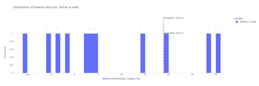
Spread Matters
One of the biggest challenges I’ve encountered is market impact. When I place a trade, I often move the entire market in my direction due to the low liquidity. This creates discrepancies between the bid, ask, mid, live, and actual trade prices. Below are examples of this from the trades I shared earlier.
The Code:
I spent a tremendous amount of time writing code to break down Polymarkets data.
strategies.py
This file contains all of the hedge opportunities that I’m monitoring.
trades = [

    {
        "trade_name": "Harris for president and all GOP electoral college margins",
        "subtitle": "This trade assumes Harris winning is the opposite of the GOP winning every category "
                    "in the electoral college. The risk is Harris could be replaced or die causing one "
                    "side of this trade to not work.",
        "side_a_trades": [
            ("2024-presidential-election-gop-wins-by-1-4", "Yes"),
            ("2024-presidential-election-gop-wins-by-5-14", "Yes"),
            ("2024-presidential-election-gop-wins-by-15-34", "Yes"),
            ("2024-presidential-election-gop-wins-by-35-64", "Yes"),
            ("2024-presidential-election-gop-wins-by-65-104", "Yes"),
            ("2024-presidential-election-gop-wins-by-105-154", "Yes"),
            ("2024-presidential-election-gop-wins-by-155-214", "Yes"),
            ("2024-presidential-election-gop-wins-by-215", "Yes"),
        ],
        "side_b_trades": [
            ("will-kamala-harris-win-the-2024-us-presidential-election", "Yes"),
        ],
        "method": "balanced"
    },


    {
        "trade_name": "DEM and REP electoral college all no",
        "subtitle": "bet no on all DEM and REP electoral college positions",
        "positions": [
            ("2024-presidential-election-gop-wins-by-215", "No"),
            ("2024-presidential-election-gop-wins-by-155-214", "No"),
            ("2024-presidential-election-gop-wins-by-65-104", "No"),
            ("2024-presidential-election-gop-wins-by-35-64", "No"),
            ("2024-presidential-election-gop-wins-by-15-34", "No"),
            ("2024-presidential-election-gop-wins-by-1-4", "No"),
            ("2024-presidential-election-gop-wins-by-5-14", "No"),
            ("2024-presidential-election-gop-wins-by-105-154", "No"),
            ("2024-presidential-election-democrats-win-by-0-4", "No"),
            ("2024-presidential-election-democrats-win-by-5-14", "No"),
            ("2024-presidential-election-democrats-win-by-15-34", "No"),
            ("2024-presidential-election-democrats-win-by-35-64", "No"),
            ("2024-presidential-election-democrats-win-by-65-104", "No"),
            ("2024-presidential-election-democrats-win-by-105-154", "No"),
            ("2024-presidential-election-democrats-win-by-155-214", "No"),
            ("2024-presidential-election-democrats-win-by-215", "No"),
        ],
        "method": "all_no"
    },

    {
        "trade_name": "DEM and GOP popular vote all no",
        "subtitle": "bet no on all DEM and GOP popular vote positions",
        "positions": [
            ("gop-wins-popular-vote-by-more-than-7", "No"),
            ("gop-wins-popular-vote-by-6-7", "No"),
            ("gop-wins-popular-vote-by-5-6", "No"),
            ("gop-wins-popular-vote-by-4-5", "No"),
            ("gop-wins-popular-vote-by-3-4", "No"),
            ("gop-wins-popular-vote-by-2-3", "No"),
            ("gop-wins-popular-vote-by-1-2", "No"),
            ("gop-wins-popular-vote-by-0-1", "No"),

            ("democrats-win-popular-vote-by-over-7", "No"),
            ("democrats-win-popular-vote-by-6-7", "No"),
            ("democrats-win-popular-vote-by-5-6", "No"),
            ("democrats-win-popular-vote-by-4-5", "No"),
            ("democrats-win-popular-vote-by-3-4", "No"),
            ("democrats-win-popular-vote-by-2-3", "No"),
            ("democrats-win-popular-vote-by-1-2", "No"),
            ("democrats-win-popular-vote-by-0-1", "No"),

        ],
        "method": "all_no"
    },

    {
        "trade_name": ""
                      "Trump for president and DEMS win presidency and popular",
        "subtitle": "If DEMS win presidency they will win popular vote so this is a direct hedge "
                    "on Trump getting elected ",
        "side_a_trades": [
            ("will-a-democrat-win-the-popular-vote-and-the-presidency", "Yes"),
        ],
        "side_b_trades": [
            ("will-donald-trump-win-the-2024-us-presidential-election", "Yes"),
        ],
        "method": "balanced"
    },

    {
        "trade_name": ""
                      "DEM win presidency hedged on Trump",
        "subtitle": "REP win presidency hedged on Kamala winning",
        "side_a_trades": [
            ("which-party-will-win-the-2024-united-states-presidential-election", "Democratic"),
        ],
        "side_b_trades": [
            ("will-donald-trump-win-the-2024-us-presidential-election", "Yes"),
        ],
        "method": "balanced"
    },

    {
        "trade_name": ""
                      "REP win presidency hedged on Kamala",
        "subtitle": "REP win presidency hedged on Kamala winning",
        "side_a_trades": [
            ("which-party-will-win-the-2024-united-states-presidential-election", "Republican"),
        ],
        "side_b_trades": [
            ("will-kamala-harris-win-the-2024-us-presidential-election", "Yes"),
        ],
        "method": "balanced"
    },

    {
        "trade_name": ""
                      "Trump popular vote hedged with popular vote margins",
        "subtitle": "Trump wins popular vote and then buy all the margins for DEMS on the popular vote",
        "side_a_trades": [
            ("will-donald-trump-win-the-popular-vote-in-the-2024-presidential-election", "Yes"),
        ],
        "side_b_trades": [
            ("democrats-win-popular-vote-by-0-1", "Yes"),
            ("democrats-win-popular-vote-by-1-2", "Yes"),
            ("democrats-win-popular-vote-by-2-3", "Yes"),
            ("democrats-win-popular-vote-by-3-4", "Yes"),
            ("democrats-win-popular-vote-by-4-5", "Yes"),
            ("democrats-win-popular-vote-by-5-6", "Yes"),
            ("democrats-win-popular-vote-by-6-7", "Yes"),
            ("democrats-win-popular-vote-by-over-7", "Yes"),

        ],
        "method": "balanced"
    },

    {
        "trade_name": ""
                      "Kamala popular vote hedged with popular vote margins",
        "subtitle": "Kamala wins popular vote and then buy all the margins for REP on the popular vote",
        "side_a_trades": [
            ("will-kamala-harris-win-the-popular-vote-in-the-2024-presidential-election", "Yes"),
        ],
        "side_b_trades": [
            ("gop-wins-popular-vote-by-0-1", "Yes"),
            ("gop-wins-popular-vote-by-1-2", "Yes"),
            ("gop-wins-popular-vote-by-2-3", "Yes"),
            ("gop-wins-popular-vote-by-3-4", "Yes"),
            ("gop-wins-popular-vote-by-4-5", "Yes"),
            ("gop-wins-popular-vote-by-5-6", "Yes"),
            ("gop-wins-popular-vote-by-6-7", "Yes"),
            ("gop-wins-popular-vote-by-more-than-7", "Yes"),

        ],
        "method": "balanced"
    },

    {
    "trade_name": "DEM popular vote all no",
    "subtitle": "bet no on all DEM popular vote positions",
    "positions": [
        ("democrats-win-popular-vote-by-over-7", "No"),
        ("democrats-win-popular-vote-by-6-7", "No"),
        ("democrats-win-popular-vote-by-5-6", "No"),
        ("democrats-win-popular-vote-by-4-5", "No"),
        ("democrats-win-popular-vote-by-3-4", "No"),
        ("democrats-win-popular-vote-by-2-3", "No"),
        ("democrats-win-popular-vote-by-1-2", "No"),
        ("democrats-win-popular-vote-by-0-1", "No"),

    ],
    "method": "all_no"
    },

    {
    "trade_name": "GOP popular vote all no",
    "subtitle": "bet no on all GOP popular vote positions",
    "positions": [
        ("gop-wins-popular-vote-by-more-than-7", "No"),
        ("gop-wins-popular-vote-by-6-7", "No"),
        ("gop-wins-popular-vote-by-5-6", "No"),
        ("gop-wins-popular-vote-by-4-5", "No"),
        ("gop-wins-popular-vote-by-3-4", "No"),
        ("gop-wins-popular-vote-by-2-3", "No"),
        ("gop-wins-popular-vote-by-1-2", "No"),
        ("gop-wins-popular-vote-by-0-1", "No"),
    ],
    "method": "all_no"
    },


    {
    "trade_name": "Trump for president and all DEM electoral college margins",
    "subtitle" : "This trade assumes Trump winning is the opposite of the DEM winning every category "
                 "in the electoral college. The risk is Trump could be replaced or die causing one "
                 "side of this trade to not work.",
    "side_a_trades": [
        ("2024-presidential-election-democrats-win-by-0-4", "Yes"),
        ("2024-presidential-election-democrats-win-by-5-14", "Yes"),
        ("2024-presidential-election-democrats-win-by-15-34", "Yes"),
        ("2024-presidential-election-democrats-win-by-35-64", "Yes"),
        ("2024-presidential-election-democrats-win-by-65-104", "Yes"),
        ("2024-presidential-election-democrats-win-by-105-154", "Yes"),
        ("2024-presidential-election-democrats-win-by-155-214", "Yes"),
        ("2024-presidential-election-democrats-win-by-215", "Yes"),
    ],
    "side_b_trades": [
        ("will-donald-trump-win-the-2024-us-presidential-election", "Yes"),
    ],
    "method": "balanced"

    },


    {
    "trade_name": "Electoral College All GOP ALL DEM YES",
    "subtitle": "This is a truely hedged trade. Bet all REP electoral college slots and bet all"
                "DEM electoral college slots",
    "side_a_trades": [
        ("2024-presidential-election-gop-wins-by-1-4", "Yes"),
        ("2024-presidential-election-gop-wins-by-5-14", "Yes"),
        ("2024-presidential-election-gop-wins-by-15-34", "Yes"),
        ("2024-presidential-election-gop-wins-by-35-64", "Yes"),
        ("2024-presidential-election-gop-wins-by-65-104", "Yes"),
        ("2024-presidential-election-gop-wins-by-105-154", "Yes"),
        ("2024-presidential-election-gop-wins-by-155-214", "Yes"),
        ("2024-presidential-election-gop-wins-by-215", "Yes"),
    ],
    "side_b_trades": [
        ("2024-presidential-election-democrats-win-by-0-4", "Yes"),
        ("2024-presidential-election-democrats-win-by-5-14", "Yes"),
        ("2024-presidential-election-democrats-win-by-15-34", "Yes"),
        ("2024-presidential-election-democrats-win-by-35-64", "Yes"),
        ("2024-presidential-election-democrats-win-by-65-104", "Yes"),
        ("2024-presidential-election-democrats-win-by-105-154", "Yes"),
        ("2024-presidential-election-democrats-win-by-155-214", "Yes"),
        ("2024-presidential-election-democrats-win-by-215", "Yes"),
    ],
    "method": "balanced"
    },

    {
    "trade_name": "DEM electoral college all no",
    "subtitle": "bet no on all DEM electoral college positions",
    "positions": [
        ("2024-presidential-election-democrats-win-by-0-4", "No"),
        ("2024-presidential-election-democrats-win-by-5-14", "No"),
        ("2024-presidential-election-democrats-win-by-15-34", "No"),
        ("2024-presidential-election-democrats-win-by-35-64", "No"),
        ("2024-presidential-election-democrats-win-by-65-104", "No"),
        ("2024-presidential-election-democrats-win-by-105-154", "No"),
        ("2024-presidential-election-democrats-win-by-155-214", "No"),
        ("2024-presidential-election-democrats-win-by-215", "No"),
    ],
    "method": "all_no"
    },

    {
    "trade_name": "REP electoral college all no",
    "subtitle": "bet no on all REP electoral college positions",
    "positions": [
        ("2024-presidential-election-gop-wins-by-1-4", "No"),
        ("2024-presidential-election-gop-wins-by-5-14", "No"),
        ("2024-presidential-election-gop-wins-by-15-34", "No"),
        ("2024-presidential-election-gop-wins-by-35-64", "No"),
        ("2024-presidential-election-gop-wins-by-65-104", "No"),
        ("2024-presidential-election-gop-wins-by-105-154", "No"),
        ("2024-presidential-election-gop-wins-by-155-214", "No"),
        ("2024-presidential-election-gop-wins-by-215", "No"),
        ],
    "method": "all_no"
    },

    {
        "trade_name": "FED Rates in Sept all no",
        "subtitle": "bet no on all FED possibilities in Sept",
        "positions": [
            ("fed-decreases-interest-rates-by-50-bps-after-september-2024-meeting", "No"),
            ("fed-decreases-interest-rates-by-25-bps-after-september-2024-meeting", "No"),
            ("no-change-in-fed-interest-rates-after-2024-september-meeting", "No"),
        ],
        "method": "all_no"
    },

    {
        "trade_name": "Balance of power all no",
        "subtitle": "bet no on some of the balance of power outcomes",
        "positions": [
            ("2024-balance-of-power-r-prez-r-senate-r-house", "No"),
            ("2024-election-democratic-presidency-and-house-republican-senate", "No"),
            ("democratic-sweep-in-2024-election", "No"),
            ("2024-balance-of-power-republican-presidency-and-senate-democratic-house", "No"),
        ],
        "method": "all_no"
    },

    {
    "trade_name": "Presidential party D President Trump",
    "subtitle": "Bet on the candidate to win and their party to lose hedging the bet",
    "side_a_trades": [
        ("which-party-will-win-the-2024-united-states-presidential-election", "Democratic"),
        ],
    "side_b_trades": [
        ("will-kamala-harris-win-the-2024-us-presidential-election", "No"),

        ],
    "method": "balanced"
    },

    {
        "trade_name": "Presidential party R President Harris",
        "subtitle": "Bet on the candidate to win and their party to lose hedging the bet",
        "side_a_trades": [
            ("which-party-will-win-the-2024-united-states-presidential-election", "Republican"),
        ],
        "side_b_trades": [
            ("will-kamala-harris-win-the-2024-us-presidential-election", "Yes"),

        ],
        "method": "balanced"
    },


    # {
    #     "trade_name": "Trump Vance ticket and vance replaced",
    #     "subtitle": "Betting on the trump and vance ticket as well as vanced replaced",
    #     "side_a_trades": [
    #         ("will-trump-vance-be-gop-ticket-on-election-day", "Yes"),
    #     ],
    #     "side_b_trades": [
    #         ("jd-vance-steps-down-as-republican-vp-nominee", "Yes"),
    #
    #     ],
    #     "method": "balanced"
    # },

    {
        "trade_name": "Other DEM wins election no and DEM wins election Yes",
        "subtitle": "Taking trade on other dem besides biden to win but then saying DEMS win Presidency",
        "side_a_trades": [
            ("democrat-other-than-biden-wins-the-presidential-election", "No"),
        ],
        "side_b_trades": [
            ("which-party-will-win-the-2024-united-states-presidential-election", "Democratic"),

        ],
        "method": "balanced"
    },

    {
        "trade_name": "538 call election no and buy predicted candidate",
        "subtitle": "538 will probably call the election correctly as indicated by the numbers. But if the day before"
                    "the election as long as you buy the same number of shares as the winning candidate cheaper than"
                    "the inverse of the price you paid for these shares you will profit",
        "side_a_trades": [
            ("will-538-correctly-call-the-presidential-election", "No"),
        ],
        "side_b_trades": [
            ("which-party-will-win-the-2024-united-states-presidential-election", "Republican"),

        ],
        "method": "balanced"
    },


    {
        "trade_name": "Nate Silver call election no and buy Nates predicted candidate",
        "subtitle": "Nate Silver will probably call the election correctly as indicated by the numbers. But if the day before"
                    "the election as long as you buy the same number of shares as the winning candidate cheaper than"
                    "the inverse of the price you paid for these shares you will profit",
        "side_a_trades": [
            ("will-nate-silver-correctly-call-the-presidential-election", "No"),
        ],
        "side_b_trades": [
            ("which-party-will-win-the-2024-united-states-presidential-election", "Republican"),

        ],
        "method": "balanced"
    },

    # {
    #     "trade_name": "DEM solid red No",
    #     "subtitle": "The main state the DEMS have a chance in is OH. So the opposite of DEMS winning a"
    #                 "solid red state, no is the DEMS actually winning the most probable state OH(10.5%)"
    #                 ". All of the rest of these states carry a < 10% chance",
    #     "side_a_trades": [
    #         ("us-presidential-election-democrats-win-a-solid-red-state", "No"),
    #     ],
    #     "side_b_trades":
    #         [
    #             # ("will-a-democrat-win-alabama-in-the-2024-us-presidential-election", "Yes"),
    #             # ("will-a-democrat-win-alaska-in-the-2024-us-presidential-election", "Yes"),
    #             # ("will-a-democrat-win-arkansas-in-the-2024-us-presidential-election", "Yes"),
    #             # ("will-a-democrat-win-idaho-in-the-2024-us-presidential-election", "Yes"),
    #             # ("will-a-democrat-win-indiana-in-the-2024-us-presidential-election", "Yes"),
    #             # ("will-a-democrat-win-iowa-in-the-2024-us-presidential-election", "Yes"),
    #             # ("will-a-democrat-win-kansas-in-the-2024-us-presidential-election", "Yes"),
    #             # ("will-a-democrat-win-kentucky-in-the-2024-us-presidential-election", "Yes"),
    #             # ("will-a-democrat-win-louisiana-in-the-2024-us-presidential-election", "Yes"),
    #             # ("will-a-democrat-win-mississippi-in-the-2024-us-presidential-election", "Yes"),
    #             # ("will-a-democrat-win-missouri-in-the-2024-us-presidential-election", "Yes"),
    #             # ("will-a-democrat-win-montana-in-the-2024-us-presidential-election", "Yes"),
    #             # ("will-a-democrat-win-nebraska-in-the-2024-us-presidential-election", "Yes"),
    #             # ("will-a-democrat-win-north-dakota-in-the-2024-us-presidential-election", "Yes"),
    #             ("will-a-democrat-win-ohio-in-the-2024-us-presidential-election", "Yes"),
    #             # ("will-a-democrat-win-oklahoma-in-the-2024-us-presidential-election", "Yes"),
    #             # ("will-a-democrat-win-south-carolina-in-the-2024-us-presidential-election", "Yes"),
    #             # ("will-a-democrat-win-south-dakota-in-the-2024-us-presidential-election", "Yes"),
    #             # ("will-a-democrat-win-tennessee-in-the-2024-us-presidential-election", "Yes"),
    #             # ("will-a-democrat-win-utah-in-the-2024-us-presidential-election", "Yes"),
    #             # ("will-a-democrat-win-west-virginia-in-the-2024-us-presidential-election", "Yes"),
    #             # ("will-a-democrat-win-wyoming-in-the-2024-us-presidential-election", "Yes")
    #         ],
    #     "method": "balanced"
    #
    # },

    # {
    #     "trade_name": "REP solid blue No",
    #     "subtitle": "The main state the REPS have a chance in is VA. So the opposite of REPS winning a"
    #                 "solid blue state, no is the REPS actually winning the most probable state VA(15%). All"
    #                 "of the rest of these states carry a < 10% chance",
    #     "side_a_trades": [
    #         ("presidential-election-republicans-win-a-solid-blue-state", "No"),
    #     ],
    #     "side_b_trades":
    #         [
    #             # ("will-a-republican-win-california-in-the-2024-us-presidential-election", "Yes"),
    #             # ("will-a-republican-win-colorado-in-the-2024-us-presidential-election", "Yes"),
    #             # ("will-a-republican-win-connecticut-in-the-2024-us-presidential-election", "Yes"),
    #             # ("will-a-republican-win-delaware-presidential-election", "Yes"),
    #             # ("will-a-republican-win-hawaii-in-the-2024-us-presidential-election", "Yes"),
    #             # ("will-a-republican-win-illinois-in-the-2024-us-presidential-election", "Yes"),
    #             # ("will-a-republican-win-maryland-in-the-2024-us-presidential-election", "Yes"),
    #             # ("will-a-republican-win-massachusetts-in-the-2024-us-presidential-election", "Yes"),
    #             # ("will-a-republican-win-new-jersey-in-the-2024-us-presidential-election", "Yes"),
    #             # ("will-a-republican-win-new-mexico-presidential-election", "Yes"),
    #             # ("will-a-republican-win-new-york-presidential-election", "Yes"),
    #             # ("will-a-republican-win-oregon-in-the-2024-us-presidential-election", "Yes"),
    #             # ("will-a-republican-win-rhode-island-in-the-2024-us-presidential-election", "Yes"),
    #             # ("will-a-republican-win-vermont-in-the-2024-us-presidential-election", "Yes"),
    #             ("will-a-republican-win-virginia-in-the-2024-us-presidential-election", "Yes"),
    #             # ("will-a-reoublican-win-washington-in-the-2024-us-presidential-election", "Yes")
    #         ],
    #     "method": "balanced"
    #
    # },


    # {
    #     "trade_name": "Trump wins every swing state yes",
    #     "subtitle": "This trade bets that trump will win every swing state(cheap). Then it bets that "
    #                 "harris will win MI(swing state). Harris is most favored to win MI 46.5/43.6 by "
    #                 "Nate Silver and 61% on Polymarket. The theory here is if Trump wins MI then he"
    #                 "should also win the other swing states given that this is the largest margin state.",
    #     "side_a_trades": [
    #         ("trump-wins-every-swing-state", "Yes"),
    #     ],
    #     "side_b_trades": [  # ("will-a-democrat-win-arizona-presidential-election", "Yes"),
    #         # ("will-a-democrat-win-georgia-presidential-election", "Yes"),
    #         ("will-a-democrat-win-michigan-presidential-election", "Yes"),
    #         # ("will-a-democrat-win-nevada-presidential-election", "Yes"),
    #         # ("will-a-democrat-win-north-carolina-presidential-election", "Yes"),
    #         # ("will-a-democrat-win-pennsylvania-presidential-election", "Yes"),
    #         # ("will-a-democrat-win-wisconsin-presidential-election", "Yes"),
    #
    #     ],
    #     "method": "balanced"
    #
    # },


    # {
    # "trade_name": "Harris wins every swing state yes",
    # "subtitle": "This trade bets that Harris will win every swing state(cheap). Then it bets that "
    #             "Trump will win GA(swing state). Trump is most favored to win GA 46.8/45.3 by "
    #             "Nate Silver and 61% on Polymarket. The theory here is if Harris wins GA then she"
    #             "should also win the other swing states given that this is the largest margin state.",            "side_a_trades": [
    #     ("will-kamala-harris-win-every-swing-state", "Yes"),
    # ],
    # "side_b_trades": [
    #     # ("will-a-democrat-win-arizona-presidential-election", "No"),
    #     ("will-a-democrat-win-georgia-presidential-election", "No"),
    #     # ("will-a-democrat-win-michigan-presidential-election", "No"),
    #     # ("will-a-democrat-win-nevada-presidential-election", "No"),
    #     # ("will-a-democrat-win-pennsylvania-presidential-election", "No"),
    #     # ("will-a-democrat-win-wisconsin-presidential-election", "No"),
    # ],
    # "method": "balanced"
    #
    # },
    #
    # {
    #     "trade_name": "REP flip Biden State",
    #     "subtitle": "test",
    #     "side_a_trades": [
    #         ("republicans-flip-a-2020-biden-state", "No"),
    #     ],
    #     "side_b_trades": [
    #         ("will-a-democrat-win-georgia-presidential-election", "No"),
    #     ],
    #     "method": "balanced"
    #
    # },
    # {
    #     "trade_name": "DEM flip Trump State",
    #     "subtitle": "test",
    #     "side_a_trades": [
    #         ("dems-flip-a-2020-trump-state", "No"),
    #     ],
    #     "side_b_trades": [
    #         ("will-a-democrat-win-north-carolina-presidential-election", "Yes"),
    #     ],
    #     "method": "balanced"
    # },

    ]
get_market_book_and_live_arb.py
This program will take your strategies and generate a nice HTML file that will constantly update the arbitrage opportunity. The output looks like this.
import os
import sys
import json
import pandas as pd
import logging
import time
from datetime import datetime
import pytz
from py_clob_client.client import ClobClient
from strategies import trades
from get_order_book import update_books_for_trades # Import the function
from dotenv import load_dotenv
import numpy as np
from get_live_price import get_live_price # Import the new live price function
import jinja2
import tempfile
import numpy as np
import subprocess
# Access the environment variables
api_key = os.getenv('API_KEY')
# Set up logging configuration
logging.basicConfig(level=logging.INFO, format='%(asctime)s - %(levelname)s - %(message)s')
# Replace with your actual host and chain ID
host = "https://clob.polymarket.com"
chain_id = 137 # Polygon Mainnet
# Initialize the ClobClient
client = ClobClient(host, key=api_key, chain_id=chain_id)
# Dictionary to cache live prices
live_price_cache = {}
# Load environment variables
load_dotenv()
def load_market_lookup():
with open('./data/market_lookup.json', 'r') as f:
market_lookup = json.load(f)
slug_to_token_id = {}
for market in market_lookup.values():
slug = market['market_slug']
slug_to_token_id[slug] = {token['outcome']: token['token_id'] for token in market['tokens']}
return slug_to_token_id
def get_actual_price(slug, outcome, user_id='JeremyRWhittaker'):
"""
Get the actual price and size from the user's latest trade for the specified slug and outcome.
"""
file_path = f'./data/user_trades/{user_id}_enriched_transactions.parquet'
if not os.path.exists(file_path):
logging.warning(f"User trades file not found: {file_path}")
return None, None
try:
df = pd.read_parquet(file_path)
except Exception as e:
logging.error(f"Failed to read user trades file: {file_path}. Error: {e}")
return None, None
# Parse 'timeStamp_erc1155' as datetime
try:
df['timeStamp_erc1155'] = pd.to_datetime(df['timeStamp_erc1155'])
except Exception as e:
logging.error(f"Failed to parse 'timeStamp_erc1155' as datetime: {e}")
return None, None
# Filter by market_slug and outcome
df_filtered = df[(df['market_slug'] == slug) & (df['outcome'] == outcome)]
if df_filtered.empty:
logging.info(f"No trades found for user {user_id} in market {slug} ({outcome})")
return None, None
# Get the row with the latest 'timeStamp_erc1155'
latest_trade = df_filtered.loc[df_filtered['timeStamp_erc1155'].idxmax()]
price = latest_trade['price_paid_per_token']
size = latest_trade['shares']
return price, size
def get_price_and_size(df, price_type):
if price_type == 'ask':
relevant_df = df[df['side'] == 'ask']
if not relevant_df.empty:
min_price_row = relevant_df.loc[relevant_df['price'].idxmin()]
return min_price_row['price'], min_price_row['size']
elif price_type == 'bid':
relevant_df = df[df['side'] == 'bid']
if not relevant_df.empty:
max_price_row = relevant_df.loc[relevant_df['price'].idxmax()]
return max_price_row['price'], max_price_row['size']
elif price_type == 'mid':
ask_df = df[df['side'] == 'ask']
bid_df = df[df['side'] == 'bid']
if not ask_df.empty and not bid_df.empty:
min_ask_price = ask_df['price'].min()
max_bid_price = bid_df['price'].max()
return (min_ask_price + max_bid_price) / 2, None
return None, None
def get_live_price(token_id, side):
cache_key = f"{token_id}_{side.upper()}"
current_time = time.time() # Get the current time in seconds since the Epoch
# Check if the price is in the cache and if it's still valid (not older than 2 minutes)
if cache_key in live_price_cache:
cached_price, timestamp = live_price_cache[cache_key]
if current_time - timestamp < 60:
return cached_price
else:
logging.info(f"Cache expired for {cache_key}. Fetching a new price.")
try:
response = client.get_last_trade_price(token_id=token_id)
price = response.get('price')
live_price_cache[cache_key] = (price, current_time) # Store the price with the current timestamp
return price
except Exception as e:
logging.error(f"Failed to fetch live price for token {token_id} on side {side}: {str(e)}")
return None
def get_live_price_from_file(token_id, side):
"""
Use the external program to fetch live prices.
"""
price = get_live_price(token_id, side)
if price is not None:
return price
else:
logging.warning(f"Failed to get live price for token ID {token_id}")
return None
def save_trade_details_with_prices(trade, trade_side_keys, price_type, output_dir, slug_to_token_id, user_id='JeremyRWhittaker'):
trade_name = trade['trade_name']
price_type_suffix = f"_{price_type}"
trade_data = []
for trade_side_key in trade_side_keys:
trade_side = trade.get(trade_side_key, [])
for slug, outcome in trade_side:
token_id = slug_to_token_id.get(slug, {}).get(outcome)
if not token_id:
logging.warning(f"Token ID not found for {slug} ({outcome})")
continue
if price_type == 'actual':
price, size = get_actual_price(slug, outcome, user_id)
if price is None:
logging.warning(f"Actual price not found for {slug} ({outcome}), skipping this pair.")
continue
elif price_type == 'live':
price = get_live_price_from_file(token_id, side='sell' if outcome.lower() == 'no' else 'buy')
size = None # We don't have size data for live prices
else:
file_name = f"{slug}_{outcome}.csv"
file_path = os.path.join('./data/book_data', file_name)
if not os.path.exists(file_path):
logging.info(f"File not found: {file_path}")
continue
df = pd.read_csv(file_path)
price, size = get_price_and_size(df, price_type)
if price is not None:
trade_data.append({
'Slug': f"{slug} ({outcome})",
'Side': trade_side_key,
'Price': float(price), # Ensure price is a float
'Size': size
})
if trade_data:
df_trade = pd.DataFrame(trade_data)
output_path = os.path.join(output_dir, f"{trade_name}{price_type_suffix}.csv")
df_trade.to_csv(output_path, index=False)
logging.info("Saved detailed trade information for %s to %s", trade_name, output_path)
def calculate_arbitrage_for_scenarios(trades, data_dir='./data/book_data', price_types=['ask', 'mid', 'live', 'bid', 'actual'], user_id='JeremyRWhittaker'):
"""
Calculate arbitrage for different price types, including 'bid' and 'actual'.
"""
arbitrage_info = {}
slug_to_token_id = load_market_lookup()
for trade in trades:
trade_name = trade['trade_name']
method = trade.get("method")
arbitrage_per_price_type = {}
if method == 'all_no':
positions = trade.get('positions', [])
if not positions:
logging.info(f"No positions found for trade: {trade_name}")
continue
elif method == 'balanced':
side_a_positions = trade.get('side_a_trades', [])
side_b_positions = trade.get('side_b_trades', [])
if not side_a_positions or not side_b_positions:
logging.info(f"No positions found for trade: {trade_name}")
continue
else:
continue
for price_type in price_types:
data_complete = True # Flag to check if all required data is available
if method == 'all_no':
# For 'all_no' method
prices = []
for slug, outcome in positions:
logging.info(f"Processing strategy: {trade_name} using {price_type} prices")
token_id = slug_to_token_id.get(slug, {}).get(outcome)
if not token_id:
logging.warning(f"Token ID not found for {slug} ({outcome}), skipping this pair.")
data_complete = False
break
if price_type == 'actual':
price, size = get_actual_price(slug, outcome, user_id)
if price is None:
logging.warning(f"Actual price not found for {slug} ({outcome}), skipping this pair.")
data_complete = False
break
elif price_type == 'live':
price = get_live_price(token_id, side='sell' if outcome.lower() == 'no' else 'buy')
else:
file_name = f"{slug}_{outcome}.csv"
file_path = os.path.join(data_dir, file_name)
if not os.path.exists(file_path):
logging.info(f"File not found: {file_path}, skipping this pair.")
data_complete = False
break
df = pd.read_csv(file_path)
price, _ = get_price_and_size(df, price_type)
if price is None:
logging.warning(f"Price not found in file for {slug} ({outcome}), skipping this pair.")
data_complete = False
break
try:
price = float(price)
except (TypeError, ValueError) as e:
logging.error(f"Failed to convert price to float for {slug} ({outcome}): {e}")
data_complete = False
break
prices.append(price)
if data_complete and prices:
max_price = max(prices)
total_winnings = sum(1 - p for p in prices) - (1 - max_price)
arb_pct = (total_winnings - max_price) * 100
logging.info(f"Total winnings: {total_winnings:.4f}, max loss: {max_price:.4f}, arb: {arb_pct:.4f}%")
arbitrage_per_price_type[price_type] = arb_pct
else:
logging.warning(f"Data incomplete for trade: {trade_name}, setting arbitrage to NaN for {price_type}.")
arbitrage_per_price_type[price_type] = np.nan
elif method == 'balanced':
# For 'balanced' method
total_cost = 0
for slug, outcome in side_a_positions + side_b_positions:
logging.info(f"Processing balanced strategy: {trade_name} using {price_type} prices")
token_id = slug_to_token_id.get(slug, {}).get(outcome)
if not token_id:
logging.warning(f"Token ID not found for {slug} ({outcome}), skipping this pair.")
data_complete = False
break
if price_type == 'actual':
price, size = get_actual_price(slug, outcome, user_id)
if price is None:
logging.warning(f"Actual price not found for {slug} ({outcome}), skipping this pair.")
data_complete = False
break
elif price_type == 'live':
price = get_live_price(token_id, side='sell' if outcome.lower() == 'no' else 'buy')
else:
file_name = f"{slug}_{outcome}.csv"
file_path = os.path.join(data_dir, file_name)
if not os.path.exists(file_path):
logging.info(f"File not found: {file_path}, skipping this pair.")
data_complete = False
break
df = pd.read_csv(file_path)
price, _ = get_price_and_size(df, price_type)
if price is None:
logging.warning(f"Price not found in file for {slug} ({outcome}), skipping this pair.")
data_complete = False
break
try:
price = float(price)
except (TypeError, ValueError) as e:
logging.error(f"Failed to convert price to float for {slug} ({outcome}): {e}")
data_complete = False
break
total_cost += price
logging.debug(f"Adding cost of {price:.4f} for {slug} ({outcome}) to total.")
if data_complete and total_cost > 0:
profit = 1 - total_cost
arb_pct = profit * 100
logging.info(f"Total cost: {total_cost:.4f}, profit: {profit:.4f}, arb: {arb_pct:.4f}%")
arbitrage_per_price_type[price_type] = arb_pct
else:
logging.warning(f"Data incomplete for trade: {trade_name}, setting arbitrage to NaN for {price_type}.")
arbitrage_per_price_type[price_type] = np.nan
if arbitrage_per_price_type:
arbitrage_info[trade_name] = arbitrage_per_price_type
logging.info(f"\nArbitrage opportunity for {trade_name}: {arbitrage_info[trade_name]}")
else:
logging.info(f"No arbitrage opportunities found for {trade_name}.")
return arbitrage_info
def get_spread_from_api(slug, outcome, slug_to_token_id):
token_id = slug_to_token_id.get(slug, {}).get(outcome)
if not token_id:
logging.warning(f"Token ID not found for {slug} ({outcome})")
return None
try:
spread_info = client.get_spread(token_id=token_id)
if spread_info and 'spread' in spread_info:
try:
spread_value = float(spread_info['spread'])
return spread_value
except ValueError:
logging.error(f"Spread value is not a float: {spread_info['spread']}")
return None
except Exception as e:
logging.error(f"Failed to fetch spread for token {token_id}: {str(e)}")
return None
def process_all_trades(trades, output_dir='./strategies', include_bid=True):
"""
Process all trades, saving the results to CSV and HTML.
"""
if not os.path.exists(output_dir):
os.makedirs(output_dir)
# Default user ID
user_id = 'JeremyRWhittaker'
# Run get_user_trade_prices.py as a subprocess with --run-once
try:
logging.info(f"Updating user trades for user: {user_id}")
subprocess.run(
['python', 'get_user_trade_prices.py', user_id, './data/strategies.py'],
check=True
)
logging.info(f"Successfully updated user trades for user: {user_id}")
except subprocess.CalledProcessError as e:
logging.error(f"Error updating user trades: {e}")
return # Exit the function if updating trades is critical
if not os.path.exists(output_dir):
os.makedirs(output_dir)
slug_to_token_id = load_market_lookup()
arbitrage_info = {}
datasets = {}
spread_info = {}
trade_descriptions = {}
# Determine the price types based on the include_bid flag
price_types = ['ask', 'mid', 'live', 'actual']
if include_bid:
price_types.append('bid')
user_id = 'JeremyRWhittaker' # Default user ID
for trade in trades:
trade_name = trade['trade_name']
trade_descriptions[trade_name] = trade.get('description', '') # Store the description
trade_datasets = {}
trade_spreads = {}
if trade['method'] == 'all_no':
for price_type in price_types:
save_trade_details_with_prices(trade, ['positions'], price_type, output_dir, slug_to_token_id, user_id)
# Load and store dataset
dataset_path = os.path.join(output_dir, f"{trade_name}_{price_type}.csv")
if os.path.exists(dataset_path):
trade_datasets[price_type] = pd.read_csv(dataset_path)
elif trade['method'] == 'balanced':
for price_type in price_types:
save_trade_details_with_prices(trade, ['side_a_trades', 'side_b_trades'], price_type, output_dir,
slug_to_token_id, user_id)
# Load and store dataset
dataset_path = os.path.join(output_dir, f"{trade_name}_{price_type}.csv")
if os.path.exists(dataset_path):
trade_datasets[price_type] = pd.read_csv(dataset_path)
# Get the spread for the trade using the token ID
for side in ['positions', 'side_a_trades', 'side_b_trades']:
trade_sides = trade.get(side, [])
for slug, outcome in trade_sides:
try:
logging.info(f"Processing trade side {side} for slug: {slug} and outcome: {outcome}")
token_id = slug_to_token_id.get(slug, {}).get(outcome)
if token_id:
logging.info(f"Token ID found for {slug} ({outcome}): {token_id}")
spread = get_spread_from_api(slug, outcome, slug_to_token_id)
if spread is not None:
trade_spreads[slug] = spread
logging.info(f"Spread for {slug} ({outcome}): {spread}")
else:
logging.warning(f"No spread found for {slug} ({outcome})")
else:
logging.warning(f"Token ID not found for {slug} ({outcome})")
except Exception as e:
logging.error(f"Error processing trade side {side} for {slug} ({outcome}): {e}", exc_info=True)
# Store the datasets and spreads
try:
logging.info(f"Storing datasets and spread information for trade: {trade_name}")
datasets[trade_name] = trade_datasets
spread_info[trade_name] = trade_spreads
except Exception as e:
logging.error(f"Error storing datasets and spreads for trade: {trade_name}: {e}", exc_info=True)
# Calculate arbitrage opportunities for all trades at once
try:
logging.info("Calculating arbitrage for all trades")
arbitrage_info = calculate_arbitrage_for_scenarios(trades, price_types=price_types, user_id=user_id)
except Exception as e:
logging.error(f"Error calculating arbitrage: {e}", exc_info=True)
# Save summary and datasets to HTML, including trade descriptions
try:
logging.info("Saving summary and datasets to HTML")
save_summary_to_html_with_datasets(arbitrage_info, datasets, spread_info, output_dir, trade_descriptions)
except Exception as e:
logging.error(f"Error saving summary and datasets to HTML: {e}", exc_info=True)
# Optionally save to CSV as well
try:
logging.info("Saving summary to CSV")
save_summary_to_csv(arbitrage_info, output_dir, datasets)
except Exception as e:
logging.error(f"Error saving summary to CSV: {e}", exc_info=True)
def save_summary_to_csv(arbitrage_info, output_dir, datasets):
"""
Save a summary of arbitrage opportunities to a CSV file.
"""
summary_data = []
# Populate summary data
for trade_name, arb_data in arbitrage_info.items():
for price_type, arb_value in arb_data.items():
summary_data.append({
'Trade Name': trade_name,
'Price Type': price_type,
'Arbitrage %': arb_value
})
if summary_data:
df_summary = pd.DataFrame(summary_data)
# Sort by Arbitrage %
df_summary.sort_values(by=['Arbitrage %'], ascending=False, inplace=True)
else:
# If no data is found, create an empty DataFrame with appropriate columns
df_summary = pd.DataFrame(columns=['Trade Name', 'Price Type', 'Arbitrage %'])
summary_path = os.path.join(output_dir, "summary.csv")
df_summary.to_csv(summary_path, index=False)
logging.info("Summary results exported to %s", summary_path)
def save_summary_to_html_with_datasets(arbitrage_info, datasets, spread_info, output_dir, trade_descriptions):
"""
Save a summary of arbitrage opportunities to an HTML file using Jinja2 templates,
with links to the corresponding detailed datasets.
"""
import numpy as np # Ensure numpy is imported
# Get the current time in Arizona time zone
arizona_tz = pytz.timezone('America/Phoenix')
run_time = datetime.now(arizona_tz).strftime('%Y-%m-%d %H:%M:%S %Z')
# Prepare data to be passed to the template
trades_summary = []
trades_list = []
for trade_name, arb_data in arbitrage_info.items():
# Get the description
description = trade_descriptions.get(trade_name, '')
# Remove the spreads from the trade name
trade_name_with_spread = trade_name # Not including spreads
# Prepare list of price types and arbitrage values for this trade
price_types_data = []
ask_arbitrage_num = None # Initialize to store ask arbitrage value
for price_type, arb_value in arb_data.items():
link_id = f"{trade_name.replace(' ', '_').replace('/', '-')}_{price_type}"
try:
arb_num = float(arb_value)
if np.isnan(arb_num):
arb_num = float('-inf')
arb_str = 'NaN'
else:
arb_str = f"{arb_num:.2f}"
except (TypeError, ValueError):
arb_num = float('-inf')
arb_str = 'NaN'
price_types_data.append({
'price_type': price_type,
'arbitrage': arb_str,
'arbitrage_num': arb_num,
'link_id': link_id
})
# Store ask arbitrage value
if price_type == 'ask':
ask_arbitrage_num = arb_num
# Get the dataset HTML
dataset = datasets.get(trade_name, {}).get(price_type)
if dataset is not None:
dataset_html = dataset.to_html(index=False)
else:
dataset_html = "<p>No data available for this trade and price type.</p>"
trades_list.append({
'trade_name': trade_name_with_spread,
'price_type': price_type,
'link_id': link_id,
'dataset_html': dataset_html
})
# Sort price_types_data, ensure 'ask' is first
price_types_data.sort(key=lambda x: 0 if x['price_type'] == 'ask' else 1)
# Add ask_arbitrage_num to trade data
trades_summary.append({
'trade_name': trade_name_with_spread,
'description': description,
'price_types': price_types_data,
'ask_arbitrage_num': ask_arbitrage_num
})
# Now sort trades_summary by 'ask_arbitrage_num' descending, handling NaN values
def sort_key(x):
ask_arb = x.get('ask_arbitrage_num')
if ask_arb is None or np.isnan(ask_arb):
return float('-inf') # Treat NaN and None as the lowest value
else:
return ask_arb
trades_summary.sort(key=sort_key, reverse=True)
# Prepare context for the template
context = {
'run_time': run_time,
'trades_summary': trades_summary,
'trades': trades_list
}
# Load the Jinja2 template with CSS styling
html_template = """
<!DOCTYPE html>
<html>
<head>
<meta http-equiv="Cache-Control" content="no-cache, no-store, must-revalidate">
<meta http-equiv="Pragma" content="no-cache">
<meta http-equiv="Expires" content="0">
<title>Arbitrage Summary</title>
<style>
body {
font-family: Arial, sans-serif;
margin: 20px;
background-color: #f9f9f9;
}
h1, h2, h3 {
color: #333;
}
table {
width: 100%;
border-collapse: collapse;
margin-bottom: 20px;
background-color: #fff;
}
th, td {
padding: 12px;
border: 1px solid #ddd;
text-align: left;
}
th {
background-color: #f4f4f4;
}
.arb-positive {
background-color: #d4edda !important; /* Light green */
}
a {
color: #3498db;
text-decoration: none;
}
a:hover {
text-decoration: underline;
}
.timestamp {
font-size: 0.9em;
color: #777;
}
.trade-section {
margin-bottom: 30px;
padding-bottom: 10px;
border-bottom: 1px solid #ccc;
}
.trade-description {
font-style: italic;
margin-bottom: 10px;
}
</style>
</head>
<body>
<h1>Arbitrage Summary</h1>
<p class="timestamp">Updated at: {{ run_time }}</p>
{% for trade in trades_summary %}
<div class="trade-section">
<h2>{{ trade.trade_name }}</h2>
{% if trade.description %}
<p class="trade-description">{{ trade.description }}</p>
{% endif %}
<table>
<thead>
<tr>
<th>Price Type</th>
<th>Arbitrage %</th>
</tr>
</thead>
<tbody>
{% for item in trade.price_types %}
<tr class="{% if item.price_type == 'ask' and item.arbitrage_num > 0 %}arb-positive{% endif %}">
<td><a href="#{{ item.link_id }}">{{ item.price_type }}</a></td>
<td>{{ item.arbitrage }}</td>
</tr>
{% endfor %}
</tbody>
</table>
</div>
{% endfor %}
{% for trade in trades %}
<h2 id="{{ trade.link_id }}">{{ trade.trade_name }} ({{ trade.price_type }})</h2>
{{ trade.dataset_html | safe }}
{% endfor %}
<script>
// Auto-reload the page every 30 seconds to reflect new updates
setInterval(function() {
window.location.reload(true); // Force reload without using the cache
}, 30000); // Reload every 30 seconds
</script>
</body>
</html>
"""
# Create a Jinja2 environment and render the template
template = jinja2.Template(html_template)
rendered_html = template.render(context)
# Write to a temporary file and then replace the original file atomically
summary_html_path = os.path.join(output_dir, "summary.html")
import tempfile
try:
# Write to a temporary file
with tempfile.NamedTemporaryFile('w', delete=False, dir=output_dir, prefix='summary_', suffix='.html') as tmp_file:
tmp_file.write(rendered_html)
temp_file_path = tmp_file.name
# Atomically replace the old file with the new file
os.replace(temp_file_path, summary_html_path)
logging.info("Summary with datasets exported to %s", summary_html_path)
except Exception as e:
logging.error(f"Error saving summary HTML file: {e}", exc_info=True)
def run_continuously(trades, output_dir='./strategies', include_bid=True, interval=300):
"""
Run the process_all_trades function every 'interval' seconds.
"""
while True:
try:
# First, update the order books
logging.info("Updating order books before processing trades.")
update_books_for_trades()
# Run the main processing function
process_all_trades(trades, output_dir=output_dir, include_bid=include_bid)
# Log the completion of one iteration
logging.info("Completed one iteration of process_all_trades.")
# Sleep for the specified interval (300 seconds = 5 minutes)
time.sleep(interval)
except Exception as e:
logging.error(f"An error occurred: {e}")
# Sleep for a bit before trying again in case of error
time.sleep(interval)
# Example usage:
if __name__ == "__main__":
run_continuously(trades, include_bid=True)
get_polygon_data.py
With this code, you can actually put in any username or wallet id and it will generate charts and graphs of that user’s trade history.
import os
import requests
import logging
import pandas as pd
import subprocess
import json
import time
from dotenv import load_dotenv
import plotly.express as px
import re
from bs4 import BeautifulSoup
from importlib import reload
import numpy as np
import argparse
import os
import subprocess
import json
import logging
import pandas as pd
from dotenv import load_dotenv
logging.basicConfig(level=logging.DEBUG, format='%(asctime)s - %(levelname)s - %(message)s')
logger = logging.getLogger(__name__)
# Load environment variables
load_dotenv("keys.env")
price_cache = {}
# EXCHANGES
CTF_EXCHANGE = '0x2791Bca1f2de4661ED88A30C99A7a9449Aa84174'
NEG_RISK_CTF_EXCHANGE = '0x4d97dcd97ec945f40cf65f87097ace5ea0476045'
# SPENDERS FOR EXCHANGES
NEG_RISK_CTF_EXCHANGE_SPENDER = '0xC5d563A36AE78145C45a50134d48A1215220f80a'
NEG_RISK_ADAPTER = '0xd91E80cF2E7be2e162c6513ceD06f1dD0dA35296'
CTF_EXCHANGE_SPENDER = '0x4bFb41d5B3570DeFd03C39a9A4D8dE6Bd8B8982E'
CACHE_EXPIRATION_TIME = 60 * 30 # Cache expiration time in seconds (5 minutes)
PRICE_CACHE_FILE = './data/live_price_cache.json'
# Dictionary to cache live prices
live_price_cache = {}
def load_price_cache():
"""Load the live price cache from a JSON file."""
if os.path.exists(PRICE_CACHE_FILE):
try:
with open(PRICE_CACHE_FILE, 'r') as file:
return json.load(file)
except json.JSONDecodeError as e:
logger.error(f"Error loading price cache: {e}")
return {}
return {}
def save_price_cache(cache):
"""Save the live price cache to a JSON file."""
with open(PRICE_CACHE_FILE, 'w') as file:
json.dump(cache, file)
def is_cache_valid(cache_entry, expiration_time=CACHE_EXPIRATION_TIME):
"""
Check if the cache entry is still valid based on the current time and expiration time.
"""
if not cache_entry:
return False
cached_time = cache_entry.get('timestamp', 0)
return (time.time() - cached_time) < expiration_time
def call_get_live_price(token_id, expiration_time=CACHE_EXPIRATION_TIME):
"""
Get live price from cache or update it if expired.
"""
logger.info(f'Getting live price for token {token_id}')
# Load existing cache
price_cache = load_price_cache()
cache_key = f"{token_id}"
# Check if cache is valid
if cache_key in price_cache and is_cache_valid(price_cache[cache_key], expiration_time):
logger.info(f'Returning cached price for {cache_key}')
return price_cache[cache_key]['price']
# If cache is expired or doesn't exist, fetch live price
try:
result = subprocess.run(
['python3', 'get_live_price.py', token_id],
stdout=subprocess.PIPE,
stderr=subprocess.PIPE,
text=True,
check=True
)
# Parse the live price from the subprocess output
output_lines = result.stdout.strip().split("\n")
live_price_line = next((line for line in output_lines if "Live price for token" in line), None)
if live_price_line:
live_price = float(live_price_line.strip().split(":")[-1].strip())
else:
logger.error("Live price not found in subprocess output.")
return None
logger.debug(f"Subprocess get_live_price output: {result.stdout}")
# Update cache with the new price and timestamp
price_cache[cache_key] = {'price': live_price, 'timestamp': time.time()}
save_price_cache(price_cache)
return live_price
except subprocess.CalledProcessError as e:
logger.error(f"Subprocess get_live_price error: {e.stderr}")
return None
except Exception as e:
logger.error(f"Error fetching live price: {str(e)}")
return None
def update_live_price_and_pl(merged_df, contract_token_id, market_slug=None, outcome=None):
"""
Calculate the live price and profit/loss (pl) for each trade in the DataFrame.
"""
# Ensure tokenID in merged_df is string
merged_df['tokenID'] = merged_df['tokenID'].astype(str)
contract_token_id = str(contract_token_id)
# Check for NaN or empty token IDs
if not contract_token_id or contract_token_id == 'nan':
logger.warning("Encountered NaN or empty contract_token_id. Skipping.")
return merged_df
# Add live_price and pl columns if they don't exist
if 'live_price' not in merged_df.columns:
merged_df['live_price'] = np.nan
if 'pl' not in merged_df.columns:
merged_df['pl'] = np.nan
# Filter rows with the same contract_token_id and outcome
merged_df['outcome'] = merged_df['outcome'].astype(str)
matching_rows = merged_df[(merged_df['tokenID'] == contract_token_id) &
(merged_df['outcome'].str.lower() == outcome.lower())]
if not matching_rows.empty:
logger.info(f'Fetching live price for token {contract_token_id}')
live_price = call_get_live_price(contract_token_id)
logger.info(f'Live price for token {contract_token_id}: {live_price}')
if live_price is not None:
try:
# Calculate profit/loss based on the live price
price_paid_per_token = matching_rows['price_paid_per_token']
total_purchase_value = matching_rows['total_purchase_value']
pl = ((live_price - price_paid_per_token) / price_paid_per_token) * total_purchase_value
# Update the DataFrame with live price and pl
merged_df.loc[matching_rows.index, 'live_price'] = live_price
merged_df.loc[matching_rows.index, 'pl'] = pl
except Exception as e:
logger.error(f"Error calculating live price and profit/loss: {e}")
else:
logger.warning(f"Live price not found for tokenID {contract_token_id}")
merged_df.loc[matching_rows.index, 'pl'] = np.nan
return merged_df
def find_token_id(market_slug, outcome, market_lookup):
"""Find the token_id based on market_slug and outcome."""
for market in market_lookup.values():
if market['market_slug'] == market_slug:
for token in market['tokens']:
if token['outcome'].lower() == outcome.lower():
return token['token_id']
return None
def fetch_data(url):
"""Fetch data from a given URL and return the JSON response."""
try:
response = requests.get(url, timeout=10) # You can specify a timeout
response.raise_for_status() # Raise an error for bad responses (4xx, 5xx)
return response.json()
except requests.exceptions.RequestException as e:
logger.error(f"Error fetching data from URL: {url}. Exception: {e}")
return None
def fetch_all_pages(api_key, token_ids, market_slug_outcome_map, csv_output_dir='./data/polymarket_trades/'):
page = 1
offset = 100
retry_attempts = 0
all_data = [] # Store all data here
while True:
url = f"https://api.polygonscan.com/api?module=account&action=token1155tx&contractaddress={NEG_RISK_CTF_EXCHANGE}&page={page}&offset={offset}&startblock=0&endblock=99999999&sort=desc&apikey={api_key}"
logger.info(f"Fetching transaction data for tokens {token_ids}, page: {page}")
data = fetch_data(url)
if data and data['status'] == '1':
df = pd.DataFrame(data['result'])
if df.empty:
logger.info("No more transactions found, ending pagination.")
break # Exit if there are no more transactions
all_data.append(df)
page += 1 # Go to the next page
else:
logger.error(f"API response error or no data found for page {page}")
if retry_attempts < 5:
retry_attempts += 1
time.sleep(retry_attempts)
else:
break
if all_data:
final_df = pd.concat(all_data, ignore_index=True) # Combine all pages
logger.info(f"Fetched {len(final_df)} transactions across all pages.")
return final_df
return None
def validate_market_lookup(token_ids, market_lookup):
valid_token_ids = []
invalid_token_ids = []
for token_id in token_ids:
market_slug, outcome = find_market_info(token_id, market_lookup)
if market_slug and outcome:
valid_token_ids.append(token_id)
else:
invalid_token_ids.append(token_id)
logger.info(f"Valid token IDs: {valid_token_ids}")
if invalid_token_ids:
logger.warning(f"Invalid or missing market info for token IDs: {invalid_token_ids}")
return valid_token_ids
def sanitize_filename(filename):
"""
Sanitize the filename by removing or replacing invalid characters.
"""
# Replace invalid characters with an underscore
return re.sub(r'[\\/*?:"<>|]', '_', filename)
def sanitize_directory(directory):
"""
Sanitize the directory name by removing or replacing invalid characters.
"""
# Replace invalid characters with an underscore
return re.sub(r'[\\/*?:"<>|]', '_', directory)
def extract_wallet_ids(leaderboard_url):
"""Scrape the Polymarket leaderboard to extract wallet IDs."""
logging.info(f"Fetching leaderboard page: {leaderboard_url}")
response = requests.get(leaderboard_url)
if response.status_code != 200:
logging.error(f"Failed to load page {leaderboard_url}, status code: {response.status_code}")
return []
logging.debug(f"Page loaded successfully, status code: {response.status_code}")
soup = BeautifulSoup(response.content, 'html.parser')
logging.debug("Page content parsed with BeautifulSoup")
wallet_ids = []
# Debug: Check if <a> tags are being found correctly
a_tags = soup.find_all('a', href=True)
logging.debug(f"Found {len(a_tags)} <a> tags in the page.")
for a_tag in a_tags:
href = a_tag['href']
logging.debug(f"Processing href: {href}")
if href.startswith('/profile/'):
wallet_id = href.split('/')[-1]
wallet_ids.append(wallet_id)
logging.info(f"Extracted wallet ID: {wallet_id}")
else:
logging.debug(f"Skipped href: {href}")
return wallet_ids
def load_market_lookup(json_path):
"""Load market lookup data from a JSON file."""
with open(json_path, 'r') as json_file:
return json.load(json_file)
def find_market_info(token_id, market_lookup):
"""Find market_slug and outcome based on tokenID."""
token_id = str(token_id) # Ensure token_id is a string
if not token_id or token_id == 'nan':
logger.warning("Token ID is NaN or empty. Skipping lookup.")
return None, None
logger.debug(f"Looking up market info for tokenID: {token_id}")
for market in market_lookup.values():
for token in market['tokens']:
if str(token['token_id']) == token_id:
logger.debug(
f"Found market info for tokenID {token_id}: market_slug = {market['market_slug']}, outcome = {token['outcome']}")
return market['market_slug'], token['outcome']
logger.warning(f"No market info found for tokenID: {token_id}")
return None, None
def fetch_data(url):
"""Fetch data from a given URL and return the JSON response."""
response = requests.get(url)
return response.json()
def save_to_csv(filename, data, headers, output_dir):
"""Save data to a CSV file in the specified output directory."""
filepath = os.path.join(output_dir, filename)
with open(filepath, 'w', newline='') as file:
writer = csv.DictWriter(file, fieldnames=headers)
writer.writeheader()
for entry in data:
writer.writerow(entry)
logger.info(f"Saved data to {filepath}")
def add_timestamps(erc1155_df, erc20_df):
"""
Rename timestamp columns and convert them from UNIX to datetime.
"""
# Rename the timestamp columns to avoid conflicts during merge
erc1155_df.rename(columns={'timeStamp': 'timeStamp_erc1155'}, inplace=True)
erc20_df.rename(columns={'timeStamp': 'timeStamp_erc20'}, inplace=True)
# Convert UNIX timestamps to datetime format
erc1155_df['timeStamp_erc1155'] = pd.to_numeric(erc1155_df['timeStamp_erc1155'], errors='coerce')
erc20_df['timeStamp_erc20'] = pd.to_numeric(erc20_df['timeStamp_erc20'], errors='coerce')
erc1155_df['timeStamp_erc1155'] = pd.to_datetime(erc1155_df['timeStamp_erc1155'], unit='s', errors='coerce')
erc20_df['timeStamp_erc20'] = pd.to_datetime(erc20_df['timeStamp_erc20'], unit='s', errors='coerce')
return erc1155_df, erc20_df
def enrich_erc1155_data(erc1155_df, market_lookup):
"""
Enrich the ERC-1155 DataFrame with market_slug and outcome based on market lookup.
"""
def get_market_info(token_id):
if pd.isna(token_id) or str(token_id) == 'nan':
return 'Unknown', 'Unknown'
for market in market_lookup.values():
for token in market['tokens']:
if str(token['token_id']) == str(token_id):
return market['market_slug'], token['outcome']
return 'Unknown', 'Unknown'
erc1155_df['market_slug'], erc1155_df['outcome'] = zip(
*erc1155_df['tokenID'].apply(lambda x: get_market_info(x))
)
return erc1155_df
def get_transaction_details_by_hash(transaction_hash, api_key, output_dir='./data/polymarket_trades/'):
"""
Fetch the transaction details by hash from Polygonscan, parse the logs, and save the flattened data as a CSV.
Args:
- transaction_hash (str): The hash of the transaction.
- api_key (str): The Polygonscan API key.
- output_dir (str): The directory to save the CSV file.
Returns:
- None: Saves the transaction details to a CSV.
"""
# Ensure output directory exists
os.makedirs(output_dir, exist_ok=True)
# Construct the API URL for fetching transaction receipt details by hash
url = f"https://api.polygonscan.com/api?module=proxy&action=eth_getTransactionReceipt&txhash={transaction_hash}&apikey={api_key}"
logger.info(f"Fetching transaction details for hash: {transaction_hash}")
logger.debug(f"Request URL: {url}")
try:
# Fetch transaction details
response = requests.get(url)
logger.debug(f"Polygonscan API response status: {response.status_code}")
if response.status_code != 200:
logger.error(f"Non-200 status code received: {response.status_code}")
return None
# Parse the JSON response
data = response.json()
logger.debug(f"Response JSON: {data}")
# Check if the status is successful
if data.get('result') is None:
logger.error(f"Error in API response: {data.get('message', 'Unknown error')}")
return None
# Extract the logs
logs = data['result']['logs']
logs_df = pd.json_normalize(logs)
# Save the logs to a CSV file for easier review
csv_filename = os.path.join(output_dir, f"transaction_logs_{transaction_hash}.csv")
logs_df.to_csv(csv_filename, index=False)
logger.info(f"Parsed logs saved to {csv_filename}")
return logs_df
except Exception as e:
logger.error(f"Exception occurred while fetching transaction details for hash {transaction_hash}: {e}")
return None
def add_financial_columns(erc1155_df, erc20_df, wallet_id, market_lookup):
"""
Merge the ERC-1155 and ERC-20 dataframes, calculate financial columns,
including whether a trade was won or lost, and fetch the latest price for each contract and tokenID.
"""
# Merge the two dataframes on the 'hash' column
merged_df = pd.merge(erc1155_df, erc20_df, how='outer', on='hash', suffixes=('_erc1155', '_erc20'))
# Convert wallet ID and columns to lowercase for case-insensitive comparison
wallet_id = wallet_id.lower()
merged_df['to_erc1155'] = merged_df['to_erc1155'].astype(str).str.lower()
merged_df['from_erc1155'] = merged_df['from_erc1155'].astype(str).str.lower()
# Remove rows where 'tokenID' is NaN or 'nan'
merged_df['tokenID'] = merged_df['tokenID'].astype(str)
merged_df = merged_df[~merged_df['tokenID'].isnull() & (merged_df['tokenID'] != 'nan')]
# Set transaction type based on wallet address
merged_df['transaction_type'] = 'other'
merged_df.loc[merged_df['to_erc1155'] == wallet_id, 'transaction_type'] = 'buy'
merged_df.loc[merged_df['from_erc1155'] == wallet_id, 'transaction_type'] = 'sell'
# Calculate the purchase price per token and total dollar value
if 'value' in merged_df.columns and 'tokenValue' in merged_df.columns:
merged_df['price_paid_per_token'] = merged_df['value'].astype(float) / merged_df['tokenValue'].astype(float)
merged_df['total_purchase_value'] = merged_df['value'].astype(float) / 10**6 # USDC has 6 decimal places
merged_df['shares'] = merged_df['total_purchase_value'] / merged_df['price_paid_per_token']
else:
logger.error("The necessary columns for calculating purchase price are missing.")
return merged_df
# Create the 'lost' and 'won' columns
merged_df['lost'] = (
(merged_df['to_erc1155'] == '0x0000000000000000000000000000000000000000') &
(merged_df['transaction_type'] == 'sell') &
(merged_df['price_paid_per_token'].isna() | (merged_df['price_paid_per_token'] == 0))
).astype(int)
merged_df['won'] = (
(merged_df['transaction_type'] == 'sell') &
(merged_df['price_paid_per_token'] == 1)
).astype(int)
merged_df.loc[merged_df['lost'] == 1, 'shares'] = 0
merged_df.loc[merged_df['lost'] == 1, 'total_purchase_value'] = 0
# Fetch live prices and calculate profit/loss (pl)
merged_df['tokenID'] = merged_df['tokenID'].astype(str)
merged_df = update_latest_prices(merged_df, market_lookup)
return merged_df
def plot_profit_loss_by_trade(df, user_info):
"""
Create a bar plot to visualize aggregated Profit/Loss (PL) by trade, with values rounded to two decimal places and formatted as currency.
Args:
df (DataFrame): DataFrame containing trade data, including 'market_slug', 'outcome', and 'pl'.
user_info (dict): Dictionary containing user information, such as username, wallet address, and other relevant details.
"""
if 'pl' not in df.columns or df['pl'].isnull().all():
logger.warning("No PL data available for plotting. Skipping plot.")
return
username = user_info.get("username", "Unknown User")
wallet_id = user_info.get("wallet_address", "N/A")
positions_value = user_info.get("positions_value", "N/A")
profit_loss = user_info.get("profit_loss", "N/A")
volume_traded = user_info.get("volume_traded", "N/A")
markets_traded = user_info.get("markets_traded", "N/A")
# Combine market_slug and outcome to create a trade identifier
df['trade'] = df['market_slug'] + ' (' + df['outcome'] + ')'
# Aggregate the Profit/Loss (pl) for each unique trade
aggregated_df = df.groupby('trade', as_index=False).agg({'pl': 'sum'})
# Round PL values to two decimal places
aggregated_df['pl'] = aggregated_df['pl'].round(2)
# Format the PL values with a dollar sign for display
aggregated_df['pl_display'] = aggregated_df['pl'].apply(lambda x: f"${x:,.2f}")
# Define a color mapping based on Profit/Loss sign
aggregated_df['color'] = aggregated_df['pl'].apply(lambda x: 'green' if x >= 0 else 'red')
# Create the plot without using the color axis
fig = px.bar(
aggregated_df,
x='trade',
y='pl',
title='',
labels={'pl': 'Profit/Loss ($)', 'trade': 'Trade (Market Slug / Outcome)'},
text='pl_display',
color='color', # Use the color column
color_discrete_map={'green': 'green', 'red': 'red'},
)
# Remove the legend if you don't want it
fig.update_layout(showlegend=False)
# Rotate x-axis labels for better readability and set the main title
fig.update_layout(
title={
'text': 'Aggregated Profit/Loss by Trade',
'y': 0.95,
'x': 0.5,
'xanchor': 'center',
'yanchor': 'top',
'font': {'size': 24}
},
xaxis_tickangle=-45,
margin=dict(t=150, l=50, r=50, b=100)
)
# Prepare the subtitle text with user information
subtitle_text = (
f"Username: {username} | Positions Value: {positions_value} | "
f"Profit/Loss: {profit_loss} | Volume Traded: {volume_traded} | "
f"Markets Traded: {markets_traded} | Wallet ID: {wallet_id}"
)
# Add the subtitle as an annotation
fig.add_annotation(
text=subtitle_text,
xref="paper",
yref="paper",
x=0.5,
y=1.02,
xanchor='center',
yanchor='top',
showarrow=False,
font=dict(size=14)
)
# Save the plot
plot_dir = "./plots/user_trades"
os.makedirs(plot_dir, exist_ok=True)
sanitized_username = sanitize_filename(username)
plot_file = os.path.join(plot_dir, f"{sanitized_username}_aggregated_profit_loss_by_trade.html")
fig.write_html(plot_file)
logger.info(f"Aggregated Profit/Loss by trade plot saved to {plot_file}")
def plot_shares_over_time(df, user_info):
"""
Create a line plot to visualize the cumulative number of shares for each token over time.
Buy orders add to the position, and sell orders subtract from it.
Args:
df (DataFrame): DataFrame containing trade data, including 'timeStamp_erc1155', 'shares', 'market_slug', 'outcome', and 'transaction_type' ('buy' or 'sell').
user_info (dict): Dictionary containing user information, such as username, wallet address, and other relevant details.
"""
if 'shares' not in df.columns or df['shares'].isnull().all():
logger.warning("No 'shares' data available for plotting. Skipping plot.")
return
username = user_info.get("username", "Unknown User")
# Ensure 'timeStamp_erc1155' is a datetime type, just in case it needs to be converted
if df['timeStamp_erc1155'].dtype != 'datetime64[ns]':
df['timeStamp_erc1155'] = pd.to_datetime(df['timeStamp_erc1155'], errors='coerce')
# Drop rows with NaN values in 'timeStamp_erc1155', 'shares', 'market_slug', 'outcome', or 'transaction_type'
df = df.dropna(subset=['timeStamp_erc1155', 'shares', 'market_slug', 'outcome', 'transaction_type'])
# Sort the dataframe by time to ensure the line chart shows the data in chronological order
df = df.sort_values(by='timeStamp_erc1155')
# Combine 'market_slug' and 'outcome' to create a unique label for each token
df['token_label'] = df['market_slug'] + " - " + df['outcome']
# Create a column for 'position_change' which adds shares for buys and subtracts shares for sells based on 'transaction_type'
df['position_change'] = df.apply(lambda row: row['shares'] if row['transaction_type'] == 'buy' else -row['shares'], axis=1)
# Group by 'token_label' and calculate the cumulative position
df['cumulative_position'] = df.groupby('token_label')['position_change'].cumsum()
# Forward fill the cumulative position to maintain it between trades
df['cumulative_position'] = df.groupby('token_label')['cumulative_position'].ffill()
# Create the line plot, grouping by 'token_label' for separate lines per token ID
fig = px.line(
df,
x='timeStamp_erc1155',
y='cumulative_position',
color='token_label', # This ensures each token ID (market_slug + outcome) gets its own line
title=f'Cumulative Shares Over Time for {username}',
labels={'timeStamp_erc1155': 'Trade Time', 'cumulative_position': 'Cumulative Position', 'token_label': 'Token (Market Slug - Outcome)'},
line_shape='linear'
)
# Update layout for better aesthetics
fig.update_layout(
title={
'text': f"Cumulative Number of Shares Over Time for {username}",
'y': 0.95,
'x': 0.5,
'xanchor': 'center',
'yanchor': 'top',
'font': {'size': 20}
},
margin=dict(t=60),
xaxis_title="Trade Time",
yaxis_title="Cumulative Number of Shares",
legend_title="Token (Market Slug - Outcome)"
)
# Save the plot
plot_dir = "./plots/user_trades"
os.makedirs(plot_dir, exist_ok=True)
sanitized_username = sanitize_filename(username)
plot_file = os.path.join(plot_dir, f"{sanitized_username}_shares_over_time.html")
fig.write_html(plot_file)
logger.info(f"Cumulative shares over time plot saved to {plot_file}")
def plot_user_trades(df, user_info):
"""Plot user trades and save plots, adjusting for trades that were lost."""
username = user_info["username"]
wallet_id = user_info["wallet_address"]
# Sanitize only the filename, not the directory
sanitized_username = sanitize_filename(username)
info_text = (
f"Username: {username} | Positions Value: {user_info['positions_value']} | "
f"Profit/Loss: {user_info['profit_loss']} | Volume Traded: {user_info['volume_traded']} | "
f"Markets Traded: {user_info['markets_traded']} | Wallet ID: {wallet_id}"
)
# Ensure the directory exists
os.makedirs("./plots/user_trades", exist_ok=True)
plot_dir = "./plots/user_trades"
# Flag loss trades where to_erc1155 is zero address, transaction_type is sell, and price_paid_per_token is NaN
df['is_loss'] = df.apply(
lambda row: (row['to_erc1155'] == '0x0000000000000000000000000000000000000000')
and (row['transaction_type'] == 'sell')
and pd.isna(row['price_paid_per_token']), axis=1)
# Set shares and total purchase value to zero for loss trades
df.loc[df['is_loss'], 'shares'] = 0
df.loc[df['is_loss'], 'total_purchase_value'] = 0
### Modify for Total Purchase Value by Market (Current holdings)
df['total_purchase_value_adjusted'] = df.apply(
lambda row: row['total_purchase_value'] if row['transaction_type'] == 'buy' else -row['total_purchase_value'],
axis=1
)
grouped_df_value = df.groupby(['market_slug']).agg({
'total_purchase_value_adjusted': 'sum',
'shares': 'sum',
}).reset_index()
# Calculate the weighted average price_paid_per_token
grouped_df_value['weighted_price_paid_per_token'] = (
grouped_df_value['total_purchase_value_adjusted'] / grouped_df_value['shares']
)
# Sort by total_purchase_value in descending order (ignoring outcome)
grouped_df_value = grouped_df_value.sort_values(by='total_purchase_value_adjusted', ascending=False)
# Format the label for the bars (removing outcome)
grouped_df_value['bar_label'] = (
"Avg Price: $" + grouped_df_value['weighted_price_paid_per_token'].round(2).astype(str)
)
fig = px.bar(
grouped_df_value,
x='market_slug',
y='total_purchase_value_adjusted',
barmode='group',
title=f"Current Total Purchase Value by Market for {username}",
labels={'total_purchase_value_adjusted': 'Current Total Purchase Value', 'market_slug': 'Market'},
text=grouped_df_value['bar_label'],
hover_data={'weighted_price_paid_per_token': ':.2f'},
)
fig.update_layout(
title={
'text': f"Current Total Purchase Value by Market for {username}",
'y': 0.95,
'x': 0.5,
'xanchor': 'center',
'yanchor': 'top',
'font': {'size': 20}
},
margin=dict(t=60),
showlegend=False # Remove the legend as you requested
)
fig.add_annotation(
text=info_text,
xref="paper", yref="paper", showarrow=False, x=0.5, y=1.05, font=dict(size=12)
)
# Save the bar plot as an HTML file
plot_file = os.path.join(plot_dir, f"{sanitized_username}_current_market_purchase_value.html")
fig.write_html(plot_file)
logger.info(f"Current market purchase value plot saved to {plot_file}")
### Modify for Trade Quantity by Market (Current holdings)
df['shares_adjusted'] = df.apply(
lambda row: row['shares'] if row['transaction_type'] == 'buy' else -row['shares'], axis=1)
grouped_df_quantity = df.groupby(['market_slug']).agg({
'shares_adjusted': 'sum',
'total_purchase_value': 'sum',
}).reset_index()
# Calculate the weighted average price_paid_per_token
grouped_df_quantity['weighted_price_paid_per_token'] = (
grouped_df_quantity['total_purchase_value'] / grouped_df_quantity['shares_adjusted']
)
grouped_df_quantity = grouped_df_quantity.sort_values(by='shares_adjusted', ascending=False)
grouped_df_quantity['bar_label'] = (
"Quantity: " + grouped_df_quantity['shares_adjusted'].round().astype(int).astype(str) + "<br>" +
"Avg Price: $" + grouped_df_quantity['weighted_price_paid_per_token'].round(2).astype(str)
)
fig = px.bar(
grouped_df_quantity,
x='market_slug',
y='shares_adjusted',
barmode='group',
title=f"Current Trade Quantity by Market for {username}",
labels={'shares_adjusted': 'Current Trade Quantity', 'market_slug': 'Market'},
text=grouped_df_quantity['bar_label'],
)
fig.update_layout(
title={
'text': f"Current Trade Quantity by Market for {username}",
'y': 0.95,
'x': 0.5,
'xanchor': 'center',
'yanchor': 'top',
'font': {'size': 20}
},
margin=dict(t=60),
showlegend=False # Remove the legend as you requested
)
fig.add_annotation(
text=info_text,
xref="paper", yref="paper", showarrow=False, x=0.5, y=1.05, font=dict(size=12)
)
# Save the trade quantity plot as an HTML file
plot_file = os.path.join(plot_dir, f"{sanitized_username}_current_market_trade_quantity.html")
fig.write_html(plot_file)
logger.info(f"Current market trade quantity plot saved to {plot_file}")
### Modify for Total Purchase Value Timeline
df['total_purchase_value_timeline_adjusted'] = df.apply(
lambda row: row['total_purchase_value'] if row['transaction_type'] == 'buy' else -row['total_purchase_value'],
axis=1
)
# Combine 'market_slug' and 'outcome' into a unique label
df['market_outcome_label'] = df['market_slug'] + ' (' + df['outcome'] + ')'
# Create the scatter plot, now coloring by 'market_outcome_label'
fig = px.scatter(
df,
x='timeStamp_erc1155',
y='total_purchase_value_timeline_adjusted',
color='market_outcome_label', # Use the combined label for market and outcome
title=f"Total Purchase Value Timeline for {username}",
labels={
'total_purchase_value_timeline_adjusted': 'Total Purchase Value',
'timeStamp_erc1155': 'Transaction Time',
'market_outcome_label': 'Market/Outcome'
},
hover_data=['market_slug', 'price_paid_per_token', 'outcome', 'hash'],
)
fig.update_layout(
title={
'text': f"Total Purchase Value Timeline for {username}",
'y': 0.95,
'x': 0.5,
'xanchor': 'center',
'yanchor': 'top',
'font': {'size': 20}
},
margin=dict(t=60)
)
fig.add_annotation(
text=info_text,
xref="paper", yref="paper", showarrow=False, x=0.5, y=1.05, font=dict(size=12)
)
# Save the updated plot
plot_file = os.path.join(plot_dir, f"{sanitized_username}_total_purchase_value_timeline_adjusted.html")
fig.write_html(plot_file)
logger.info(f"Total purchase value timeline plot saved to {plot_file}")
def plot_total_purchase_value(df, user_info):
"""Create and save a scatter plot for total purchase value, accounting for buy and sell transactions."""
# Ensure the directory exists
os.makedirs("./plots/user_trades", exist_ok=True)
plot_dir = "./plots/user_trades"
username = user_info["username"]
wallet_id = user_info["wallet_address"]
# Sanitize only the filename, not the directory
sanitized_username = sanitize_filename(username)
info_text = (
f"Username: {username} | Positions Value: {user_info['positions_value']} | "
f"Profit/Loss: {user_info['profit_loss']} | Volume Traded: {user_info['volume_traded']} | "
f"Markets Traded: {user_info['markets_traded']} | Wallet ID: {wallet_id}"
)
# Flag loss trades where to_erc1155 is zero address, transaction_type is sell, and price_paid_per_token is NaN
df['is_loss'] = df.apply(
lambda row: (row['to_erc1155'] == '0x0000000000000000000000000000000000000000')
and (row['transaction_type'] == 'sell')
and pd.isna(row['price_paid_per_token']), axis=1)
# Set shares and total purchase value to zero for loss trades
df.loc[df['is_loss'], 'shares'] = 0
df.loc[df['is_loss'], 'total_purchase_value'] = 0
# Adjust the total purchase value based on the transaction type
df['total_purchase_value_adjusted'] = df.apply(
lambda row: row['total_purchase_value'] if row['transaction_type'] == 'buy' else -row['total_purchase_value'],
axis=1
)
# Create the scatter plot for total purchase value over time
fig = px.scatter(
df,
x='timeStamp_erc1155', # Assuming this is the correct timestamp field
y='total_purchase_value_adjusted', # Adjusted values for buys and sells
color='market_slug', # Use market_slug with outcome as the color
title=f"Current Purchase Value Timeline for {username}", # Update title to reflect "current"
labels={'total_purchase_value_adjusted': 'Adjusted Purchase Value ($)', 'timeStamp_erc1155': 'Transaction Time'},
hover_data=['market_slug', 'price_paid_per_token', 'outcome', 'hash'],
)
# Adjust title positioning and font size
fig.update_layout(
title={
'text': f"Current Purchase Value Timeline for {username}", # Update to "Current"
'y': 0.95,
'x': 0.5,
'xanchor': 'center',
'yanchor': 'top',
'font': {'size': 20}
},
margin=dict(t=60)
)
fig.add_annotation(
text=info_text,
xref="paper", yref="paper", showarrow=False, x=0.5, y=1.05, font=dict(size=12)
)
# Save the scatter plot as an HTML file
plot_file = os.path.join(plot_dir, f"{sanitized_username}_current_purchase_value_timeline.html")
fig.write_html(plot_file)
logger.info(f"Current purchase value timeline plot saved to {plot_file}")
def create_and_save_pie_chart(df, user_info):
"""Create and save a pie chart for user's current holdings."""
# Ensure the directory exists
os.makedirs("./plots/user_trades", exist_ok=True)
plot_dir = "./plots/user_trades"
username = user_info["username"]
wallet_id = user_info["wallet_address"]
sanitized_username = sanitize_filename(username)
info_text = (
f"Username: {username} | Positions Value: {user_info['positions_value']} | "
f"Profit/Loss: {user_info['profit_loss']} | Volume Traded: {user_info['volume_traded']} | "
f"Markets Traded: {user_info['markets_traded']} | Wallet ID: {wallet_id}"
)
# Flag loss trades where to_erc1155 is zero address, transaction_type is sell, and price_paid_per_token is NaN
df['is_loss'] = df.apply(
lambda row: (row['to_erc1155'] == '0x0000000000000000000000000000000000000000')
and (row['transaction_type'] == 'sell')
and pd.isna(row['price_paid_per_token']), axis=1)
# Set shares and total purchase value to zero for loss trades
df.loc[df['is_loss'], 'shares'] = 0
df['shares_adjusted'] = df.apply(
lambda row: row['shares'] if row['transaction_type'] == 'buy' else -row['shares'], axis=1)
holdings = df.groupby('market_slug').agg({'shares_adjusted': 'sum'}).reset_index()
holdings = holdings.sort_values('shares_adjusted', ascending=False)
threshold = 0.02
large_slices = holdings[holdings['shares_adjusted'] > holdings['shares_adjusted'].sum() * threshold]
small_slices = holdings[holdings['shares_adjusted'] <= holdings['shares_adjusted'].sum() * threshold]
if not small_slices.empty:
other_sum = small_slices['shares_adjusted'].sum()
others_df = pd.DataFrame([{'market_slug': 'Others', 'shares_adjusted': other_sum}])
large_slices = pd.concat([large_slices, others_df], ignore_index=True)
fig = px.pie(
large_slices,
names='market_slug',
values='shares_adjusted',
title=f"Current Holdings Distribution by Market for {username}",
)
fig.update_layout(
title={
'text': f"Current Holdings Distribution by Market for {username}",
'y': 0.95,
'x': 0.5,
'xanchor': 'center',
'yanchor': 'top',
'font': {'size': 20}
},
margin=dict(t=60)
)
fig.add_annotation(
text=info_text,
xref="paper", yref="paper", showarrow=False, x=0.5, y=1.05, font=dict(size=12)
)
# Save the pie chart as an HTML file
plot_file = os.path.join(plot_dir, f"{sanitized_username}_current_holdings_pie_chart.html")
fig.write_html(plot_file)
logger.info(f"Current holdings pie chart saved to {plot_file}")
def create_and_save_treemap(df, user_info):
"""Create and save a treemap for user's current holdings."""
plot_dir = './plots/user_trades'
username = user_info["username"]
wallet_id = user_info["wallet_address"]
sanitized_username = sanitize_filename(username)
info_text = (
f"Username: {username} | Positions Value: {user_info['positions_value']} | "
f"Profit/Loss: {user_info['profit_loss']} | Volume Traded: {user_info['volume_traded']} | "
f"Markets Traded: {user_info['markets_traded']} | Wallet ID: {wallet_id}"
)
# Flag loss trades where to_erc1155 is zero address, transaction_type is sell, and price_paid_per_token is NaN
df['is_loss'] = df.apply(
lambda row: (row['to_erc1155'] == '0x0000000000000000000000000000000000000000')
and (row['transaction_type'] == 'sell')
and pd.isna(row['price_paid_per_token']), axis=1)
# Set shares and total purchase value to zero for loss trades
df.loc[df['is_loss'], 'shares'] = 0
# Adjust shares based on transaction type (buy vs sell)
df['shares_adjusted'] = df.apply(
lambda row: row['shares'] if row['transaction_type'] == 'buy' else -row['shares'], axis=1)
# Group by market_slug and outcome for treemap
holdings = df.groupby(['market_slug', 'outcome']).agg({'shares_adjusted': 'sum'}).reset_index()
# Create the treemap
fig = px.treemap(
holdings,
path=['market_slug', 'outcome'],
values='shares_adjusted',
title=f"Current Holdings Distribution by Market and Outcome for {username}",
)
# Adjust title positioning and font size
fig.update_layout(
title={
'text': f"Current Holdings Distribution by Market and Outcome for {username}",
'y': 0.95,
'x': 0.5,
'xanchor': 'center',
'yanchor': 'top',
'font': {'size': 20}
},
margin=dict(t=60)
)
fig.add_annotation(
text=info_text,
xref="paper", yref="paper", showarrow=False, x=0.5, y=1.05, font=dict(size=12)
)
# Save the treemap as an HTML file
plot_file = os.path.join(plot_dir, f"{sanitized_username}_current_holdings_treemap.html")
fig.write_html(plot_file)
logger.info(f"Current holdings treemap saved to {plot_file}")
def update_latest_prices(merged_df, market_lookup):
"""
Fetch and update the latest prices for each contract and tokenID pair in the merged_df,
and calculate profit/loss (pl) based on the live price.
"""
# Ensure 'pl' column exists in the DataFrame
if 'pl' not in merged_df.columns:
merged_df['pl'] = np.nan # Import numpy as np at the top of your script
# Ensure tokenID is a string and filter out NaN tokenIDs
merged_df['tokenID'] = merged_df['tokenID'].astype(str)
merged_df = merged_df[~merged_df['tokenID'].isnull() & (merged_df['tokenID'] != 'nan')]
unique_contract_token_pairs = merged_df[['contractAddress_erc1155', 'tokenID']].drop_duplicates()
for contract_address, token_id in unique_contract_token_pairs.itertuples(index=False):
# Ensure token_id is a string
token_id_str = str(token_id)
if not token_id_str or token_id_str == 'nan':
logger.warning("Encountered NaN or empty token_id. Skipping.")
continue
# Find market_slug and outcome using the market_lookup
market_slug, outcome = find_market_info(token_id_str, market_lookup)
if market_slug and outcome:
# Update live price and pl in the DataFrame
merged_df = update_live_price_and_pl(merged_df, token_id_str, market_slug=market_slug, outcome=outcome)
else:
logger.warning(f"Market info not found for token ID: {token_id_str}. Skipping PL calculation for these rows.")
# Optionally, set 'pl' to 0 or np.nan for these rows
merged_df.loc[merged_df['tokenID'] == token_id_str, 'pl'] = np.nan
return merged_df
def call_get_user_profile(wallet_id):
"""
Call subprocess to get user profile data by wallet_id.
"""
if not wallet_id:
logger.error("No wallet ID provided.")
return None
try:
logger.info(f"Calling subprocess to fetch user profile for wallet ID: {wallet_id}")
# Execute get_user_profile.py using subprocess and pass wallet_id
result = subprocess.run(
['python3', 'get_user_profile.py', wallet_id], # Make sure wallet_id is passed as an argument
stdout=subprocess.PIPE,
stderr=subprocess.PIPE,
check=True,
text=True,
timeout=30 # Set a timeout for the subprocess
)
logger.debug(f"Subprocess stdout: {result.stdout}")
logger.debug(f"Subprocess stderr: {result.stderr}")
# Parse the JSON response from stdout
user_data = json.loads(result.stdout)
return user_data
except subprocess.TimeoutExpired:
logger.error(f"Subprocess timed out when fetching user profile for wallet ID: {wallet_id}")
return None
except subprocess.CalledProcessError as e:
logger.error(f"Subprocess error when fetching user profile for wallet ID {wallet_id}: {e.stderr}")
return None
except json.JSONDecodeError as e:
logger.error(f"Failed to parse JSON from subprocess for wallet ID {wallet_id}: {e}")
return None
def replace_hex_values(df, columns):
"""
Replace specific hex values in the given columns with their corresponding names.
Args:
- df (pd.DataFrame): The DataFrame containing the transaction data.
- columns (list): List of column names where the hex values should be replaced.
Returns:
- pd.DataFrame: The DataFrame with the replaced values.
"""
# Mapping of hex values to their corresponding names
replacement_dict = {
'0x2791Bca1f2de4661ED88A30C99A7a9449Aa84174': 'CTF_EXCHANGE',
'0x4d97dcd97ec945f40cf65f87097ace5ea0476045': 'NEG_RISK_CTF_EXCHANGE',
'0xC5d563A36AE78145C45a50134d48A1215220f80a': 'NEG_RISK_CTF_EXCHANGE_SPENDER',
'0xd91E80cF2E7be2e162c6513ceD06f1dD0dA35296': 'NEG_RISK_ADAPTER',
'0x4bFb41d5B3570DeFd03C39a9A4D8dE6Bd8B8982E': 'CTF_EXCHANGE_SPENDER',
}
for column in columns:
if column in df.columns:
df[column] = df[column].replace(replacement_dict)
return df
def process_wallet_data(wallet_addresses, api_key, plot=True, latest_price_mode=False):
"""
Processes user wallet data to generate user transaction information. If `latest_price_mode` is set to True,
the function will only retrieve the latest prices for tokens without generating user reports.
Args:
- wallet_addresses (list): List of wallet addresses to process.
- api_key (str): The Polygonscan API key.
- plot (bool): Whether to generate plots for the user data.
- latest_price_mode (bool): If True, only retrieve the latest transaction prices for the given wallets.
"""
# Load environment variables
load_dotenv("keys.env")
# Ensure the output directory exists
output_dir = './data/user_trades/'
os.makedirs(output_dir, exist_ok=True)
# Load the market lookup JSON data
market_lookup_path = './data/market_lookup.json'
market_lookup = load_market_lookup(market_lookup_path)
for wallet_address in wallet_addresses:
# Fetch user info (username) based on wallet ID
user_info = call_get_user_profile(wallet_address) # Pass wallet_address to the function
username = user_info['username'] if user_info else "Unknown"
# Sanitize the username to create a valid filename
sanitized_username = sanitize_filename(username)
logger.info(f"Processing wallet for user: {username}")
# API URLs for ERC-20 and ERC-1155 transactions
erc20_url = f"https://api.polygonscan.com/api?module=account&action=tokentx&address={wallet_address}&startblock=0&endblock=99999999&sort=asc&apikey={api_key}"
erc1155_url = f"https://api.polygonscan.com/api?module=account&action=token1155tx&address={wallet_address}&startblock=0&endblock=99999999&sort=asc&apikey={api_key}"
# Fetch ERC-20 and ERC-1155 transactions
erc20_response = fetch_data(erc20_url)
erc1155_response = fetch_data(erc1155_url)
if erc20_response['status'] == '1' and erc1155_response['status'] == '1':
erc20_data = erc20_response['result']
erc1155_data = erc1155_response['result']
# Convert data to DataFrames
erc20_df = pd.DataFrame(erc20_data)
erc1155_df = pd.DataFrame(erc1155_data)
# Enrich ERC-1155 data with market_slug and outcome
erc1155_df = enrich_erc1155_data(erc1155_df, market_lookup)
# Add timestamps
erc1155_df, erc20_df = add_timestamps(erc1155_df, erc20_df)
# Merge and add financial columns
merged_df = add_financial_columns(erc1155_df, erc20_df, wallet_address, market_lookup)
if 'pl' in merged_df.columns:
logger.info(f"'pl' column exists with {merged_df['pl'].count()} non-null values.")
else:
logger.error("'pl' column does not exist in merged_df after update_latest_prices.")
# Replace hex values with the corresponding names
columns_to_replace = ['contractAddress_erc1155', 'from_erc1155', 'to_erc1155']
merged_df = replace_hex_values(merged_df, columns_to_replace)
# Save the merged and enriched data
output_file = f'{output_dir}{sanitized_username}_enriched_transactions.csv'
merged_df.to_csv(output_file, index=False)
logger.info(f"Enriched data saved to {output_file}")
# Check if 'pl' column exists and has non-null values
if 'pl' in merged_df.columns and merged_df['pl'].notnull().any():
logger.info(f"'pl' column exists with {merged_df['pl'].count()} non-null values.")
if not latest_price_mode:
# Generate and save the Profit/Loss by trade plot
plot_profit_loss_by_trade(merged_df, user_info)
else:
logger.warning(f"'pl' column is missing or empty for user {username}. Skipping PL plot.")
logger.info("Data processing completed.")
def call_scrape_wallet_ids(top_volume=True, top_profit=True):
"""
Scrape leaderboard and return wallet IDs based on top volume or top profit.
Args:
- top_volume (bool): Whether to fetch top volume users.
- top_profit (bool): Whether to fetch top profit users.
Returns:
- List of wallet IDs.
"""
wallet_ids = []
# Construct the command to call get_leaderboard_wallet_ids.py with appropriate flags
command = ['python3', 'get_leaderboard_wallet_ids.py']
if top_volume:
command.append('--top-volume')
if top_profit:
command.append('--top-profit')
try:
# Run the script with the constructed command
result = subprocess.run(
command,
stdout=subprocess.PIPE,
stderr=subprocess.PIPE,
check=True,
text=True
)
logger.debug(f"Leaderboard wallet script stdout: {result.stdout}")
# Parse the output as JSON and extend the wallet_ids list
wallet_ids.extend(json.loads(result.stdout))
except subprocess.CalledProcessError as e:
logger.error(f"Error running get_leaderboard_wallet_ids.py: {e.stderr}")
except json.JSONDecodeError as json_err:
logger.error(f"Failed to parse JSON from get_leaderboard_wallet_ids.py: {json_err}")
# Log the combined wallet IDs
logger.info(f"Fetched {len(wallet_ids)} wallet IDs based on volume/profit flags.")
return wallet_ids
def process_and_plot_user_data(wallet_addresses, api_key, plot=True, latest_price_mode=False):
"""
Process wallet data for each user, calculate financial data, and optionally generate plots.
Args:
wallet_addresses (list): List of wallet addresses.
api_key (str): Polygonscan API key.
plot (bool): Whether to generate plots for the user data.
latest_price_mode (bool): If True, only retrieve the latest prices, no plotting.
"""
# Load market lookup data
market_lookup_path = './data/market_lookup.json'
market_lookup = load_market_lookup(market_lookup_path)
# Define the columns to keep
columns_to_keep = [
'timeStamp_erc1155', 'tokenID', 'tokenValue', 'market_slug', 'outcome',
'value', 'tokenDecimal', 'transaction_type', 'price_paid_per_token',
'total_purchase_value', 'shares', 'lost', 'won', 'pl', 'live_price'
]
for wallet_address in wallet_addresses:
# Fetch user info (username) based on wallet ID
user_info = call_get_user_profile(wallet_address)
username = user_info.get('username', "Unknown")
logger.info(f"Processing wallet for user: {username} ({wallet_address})")
# Fetch ERC-20 and ERC-1155 transactions
erc20_df, erc1155_df = fetch_user_transactions(wallet_address, api_key)
if erc20_df is not None and erc1155_df is not None:
# Enrich ERC-1155 data with market_slug and outcome
erc1155_df = enrich_erc1155_data(erc1155_df, market_lookup)
# Add timestamps
erc1155_df, erc20_df = add_timestamps(erc1155_df, erc20_df)
# Merge and add financial columns
merged_df = add_financial_columns(erc1155_df, erc20_df, wallet_address, market_lookup)
# Check for Profit/Loss data
if 'pl' in merged_df.columns and merged_df['pl'].notnull().any():
if not latest_price_mode and plot:
# Generate all plots for the user
generate_all_user_plots(merged_df, user_info)
# Save the merged and enriched data
sanitized_username = sanitize_filename(username)
output_dir = './data/user_trades/'
os.makedirs(output_dir, exist_ok=True)
# Save to Parquet (default format)
output_file_parquet = f'{output_dir}{sanitized_username}_enriched_transactions.parquet'
merged_df.to_parquet(output_file_parquet, index=False)
logger.info(f"Enriched data saved to {output_file_parquet}")
# Save to CSV
# Keep only the specified columns and sort by timeStamp_erc1155
merged_df = merged_df[columns_to_keep].sort_values(by='timeStamp_erc1155', ascending=True)
output_file_csv = f'{output_dir}{sanitized_username}_enriched_transactions.csv'
merged_df.to_csv(output_file_csv, index=False)
logger.info(f"Enriched data saved to {output_file_csv}")
else:
logger.warning(f"Profit/Loss column missing or empty for user: {username}")
else:
logger.error(f"Failed to fetch transaction data for wallet: {wallet_address}")
def generate_all_user_plots(merged_df, user_info):
"""
Generate all necessary plots for a user.
Args:
merged_df (DataFrame): The merged DataFrame with user transactions and financial info.
user_info (dict): Dictionary containing user information.
"""
# Generate Profit/Loss by Trade plot
plot_profit_loss_by_trade(merged_df, user_info)
# Generate Shares Over Time plot
plot_shares_over_time(merged_df, user_info)
# Generate Total Purchase Value by Market plot
plot_user_trades(merged_df, user_info)
# Generate Pie Chart for Holdings
create_and_save_pie_chart(merged_df, user_info)
# Generate Treemap for Holdings
create_and_save_treemap(merged_df, user_info)
logger.info(f"All plots generated for user: {user_info['username']}")
def fetch_user_transactions(wallet_address, api_key):
"""
Fetch ERC-20 and ERC-1155 transaction data for a user with pagination.
Args:
wallet_address (str): Wallet address to fetch transactions for.
api_key (str): Polygonscan API key.
Returns:
(DataFrame, DataFrame): DataFrames for ERC-20 and ERC-1155 transactions.
"""
def fetch_paginated_data(url):
"""
Fetch paginated data from the provided URL.
Args:
url (str): Base URL for the API request.
Returns:
DataFrame: DataFrame with all paginated results.
"""
page = 1
offset = 1000 # Set the offset/page size based on the API's limits (e.g., 1000)
all_data = []
while True:
paginated_url = f"{url}&page={page}&offset={offset}"
data = fetch_data(paginated_url)
if data and data['status'] == '1' and len(data['result']) > 0:
all_data.extend(data['result'])
page += 1
else:
break # Stop if no more data is returned
return pd.DataFrame(all_data)
# Fetch ERC-20 transactions with pagination
erc20_url = (f"https://api.polygonscan.com/api"
f"?module=account"
f"&action=tokentx"
f"&address={wallet_address}"
f"&startblock=0"
f"&endblock=99999999"
f"&sort=desc"
f"&apikey={api_key}")
erc20_df = fetch_paginated_data(erc20_url)
# Fetch ERC-1155 transactions with pagination
erc1155_url = (f"https://api.polygonscan.com/api"
f"?module=account"
f"&action=token1155tx"
f"&address={wallet_address}"
f"&startblock=0"
f"&endblock=99999999"
f"&sort=desc"
f"&apikey={api_key}")
erc1155_df = fetch_paginated_data(erc1155_url)
if not erc20_df.empty and not erc1155_df.empty:
return erc20_df, erc1155_df
else:
return None, None
def fetch_wallet_addresses(skip_leaderboard, top_volume, top_profit):
"""
Fetch wallet addresses based on leaderboard data or manual input.
Args:
skip_leaderboard (bool): Whether to skip leaderboard fetching.
top_volume (bool): Fetch top volume users.
top_profit (bool): Fetch top profit users.
Returns:
list: A list of wallet addresses to process.
"""
# Manually specified wallet addresses
manual_wallet_ids = [
'0x76527252D7FEd00dC4D08d794aFa1cCC36069C2a',
# Add more wallet IDs as needed
]
if not skip_leaderboard:
leaderboard_wallet_ids = call_scrape_wallet_ids(top_volume=top_volume, top_profit=top_profit)
wallet_addresses = list(set(manual_wallet_ids + leaderboard_wallet_ids)) # Remove duplicates
else:
wallet_addresses = manual_wallet_ids
return wallet_addresses
def main(wallet_addresses=None, skip_leaderboard=False, top_volume=False, top_profit=False, plot=True, latest_price_mode=False):
"""
Main function to process wallet data and generate plots.
Args:
wallet_addresses (list): A list of wallet addresses to process (if provided).
skip_leaderboard (bool): Whether to skip fetching leaderboard data.
top_volume (bool): Whether to fetch top volume users.
top_profit (bool): Whether to fetch top profit users.
plot (bool): Whether to generate plots for the user data.
latest_price_mode (bool): If True, only retrieve the latest prices, no plotting.
"""
# Load environment variables
load_dotenv("keys.env")
api_key = os.getenv('POLYGONSCAN_API_KEY')
if not wallet_addresses:
# Fetch wallet addresses if not provided
wallet_addresses = fetch_wallet_addresses(skip_leaderboard, top_volume, top_profit)
# Process wallet data and optionally generate plots
process_and_plot_user_data(wallet_addresses, api_key, plot=plot, latest_price_mode=latest_price_mode)
if __name__ == "__main__":
# Use argparse to accept command-line arguments
parser = argparse.ArgumentParser(description='Process wallet data for specific wallet addresses.')
parser.add_argument(
'--wallets',
nargs='+', # This will accept multiple wallet IDs
help='List of wallet addresses to process.'
)
parser.add_argument('--skip-leaderboard', action='store_true', help='Skip leaderboard fetching.')
parser.add_argument('--top-volume', action='store_true', help='Fetch top volume users.')
parser.add_argument('--top-profit', action='store_true', help='Fetch top profit users.')
parser.add_argument('--no-plot', action='store_true', help='Disable plot generation.')
parser.add_argument('--latest-price-mode', action='store_true',
help='Only retrieve the latest prices, no plotting.')
args = parser.parse_args()
# Call the main function with the parsed arguments
main(
wallet_addresses=args.wallets,
skip_leaderboard=args.skip_leaderboard,
top_volume=args.top_volume,
top_profit=args.top_profit,
plot=not args.no_plot,
latest_price_mode=args.latest_price_mode
)
plot_arb.py
This code will take all of your strategies and then plot the arb into a nice HTML file for review.
import os
import subprocess
import pandas as pd
import plotly.graph_objects as go
from plotly.subplots import make_subplots
import time
import pytz
import logging
from strategies import trades
import json
# Setup logging
logging.basicConfig(level=logging.INFO, format='%(asctime)s - %(levelname)s - %(message)s')
plot_dir = "./plots/"
os.makedirs(plot_dir, exist_ok=True)
def load_market_lookup():
"""
Loads the market lookup JSON and maps slugs to token IDs based on outcomes.
"""
with open('./data/market_lookup.json', 'r') as f:
market_lookup = json.load(f)
slug_to_token_id = {}
for market in market_lookup.values():
slug = market['market_slug']
slug_to_token_id[slug] = {token['outcome']: token['token_id'] for token in market['tokens']}
return slug_to_token_id
def run_get_trade_slugs_to_parquet(token_id, market_slug, outcome):
"""
Runs the get_trade_slugs_to_parquet.py script with the specified arguments to fetch and save timeseries data.
"""
script_path = os.path.join(os.path.dirname(os.path.abspath(__file__)), 'get_trade_slugs_to_parquet.py')
try:
result = subprocess.run(["python3", script_path, token_id, market_slug, outcome], capture_output=True, text=True)
if result.returncode != 0:
logging.error(f"Error running get_trade_slugs_to_parquet.py: {result.stderr}")
raise RuntimeError("Failed to run get_trade_slugs_to_parquet.py")
logging.info("get_trade_slugs_to_parquet.py ran successfully.")
except Exception as e:
logging.exception("Failed to run the script.")
def process_and_fetch_data(trade_slug, outcome):
"""
Fetches the token_id for the given trade_slug and outcome and runs the get_trade_slugs_to_parquet function.
"""
market_lookup = load_market_lookup() # Load the market lookup from JSON
if trade_slug in market_lookup and outcome in market_lookup[trade_slug]:
token_id = market_lookup[trade_slug][outcome]
run_get_trade_slugs_to_parquet(token_id, trade_slug, outcome)
else:
logging.error(f"Slug '{trade_slug}' or outcome '{outcome}' not found in the lookup.")
def plot_parquet(file_path):
"""
Plots the data from a Parquet file and saves the plot as an HTML file.
"""
try:
df = pd.read_parquet(file_path)
if 'timestamp' in df.columns and 'price' in df.columns:
fig = go.Figure()
fig.add_trace(go.Scatter(x=df['timestamp'], y=df['price'], mode='lines',
name=os.path.basename(file_path).replace('.parquet', '')))
output_file = os.path.join(plot_dir, os.path.basename(file_path).replace('.parquet', '.html'))
fig.write_html(output_file)
logging.info(f"Plot saved to {output_file}")
else:
logging.warning(f"Data in {file_path} does not contain expected columns 'timestamp' and 'price'")
except Exception as e:
logging.exception(f"Failed to plot data from Parquet file {file_path}")
def plot_trade_sides(trade_name, subtitle, side_a_trades=None, side_b_trades=None, positions=None, method="balanced", timezone='America/Phoenix', plot_last_x_days=14):
"""
Plots cumulative data for two sides of a trade, the arbitrage percentage, and individual slug data.
Includes a subtitle for the chart. Only the last plot_last_x_days days of data will be plotted.
:param trade_name: The name of the trade.
:param subtitle: The subtitle or hypothesis to be displayed below the title.
:param side_a_trades: List of tuples for side A trades, where each tuple is (slug, 'Yes' or 'No').
:param side_b_trades: List of tuples for side B trades, where each tuple is (slug, 'Yes' or 'No').
:param positions: List of positions (slug, 'No') for the 'all_no' method.
:param method: The method to use for arbitrage calculation ("balanced" or "all_no").
:param timezone: The desired timezone for displaying timestamps. Default is 'America/Phoenix'.
:param plot_last_x_days: The number of days of data to display in the plot. Default is 14.
"""
def convert_timezone(df, timezone):
df['timestamp'] = pd.to_datetime(df['timestamp'], utc=True)
df['timestamp'] = df['timestamp'].dt.tz_convert(timezone)
return df
def truncate_data_for_plotting(df, plot_last_x_days):
if not df.empty:
last_timestamp = df['timestamp'].max()
cutoff_timestamp = last_timestamp - pd.Timedelta(days=plot_last_x_days)
df = df[df['timestamp'] >= cutoff_timestamp]
return df
def aggregate_side(trades):
combined_df = pd.DataFrame()
missing_files = []
missing_columns = []
for slug, outcome in trades:
file_path = f"./data/historical/{slug}_{outcome}.parquet"
if os.path.exists(file_path):
df = pd.read_parquet(file_path)
if 'timestamp' in df.columns and 'price' in df.columns:
df = convert_timezone(df, timezone)
df = df.drop_duplicates(subset='timestamp')
df = df.set_index('timestamp').resample('min').ffill().reset_index()
if combined_df.empty:
combined_df = df[['timestamp', 'price']].copy()
else:
combined_df = pd.merge(combined_df, df[['timestamp', 'price']], on='timestamp', how='outer')
combined_df['price'] = combined_df['price_x'].fillna(0) + combined_df['price_y'].fillna(0)
combined_df = combined_df[['timestamp', 'price']]
else:
missing_columns.append(file_path)
print(f"Data in {file_path} does not contain expected columns 'timestamp' and 'price'")
return None, missing_files, missing_columns
else:
missing_files.append(file_path)
print(f"File {file_path} does not exist.")
return None, missing_files, missing_columns
return truncate_data_for_plotting(combined_df, plot_last_x_days), missing_files, missing_columns
def aggregate_positions(positions):
combined_df = pd.DataFrame()
missing_files = []
missing_columns = []
for slug, outcome in positions:
file_path = f"./data/historical/{slug}_{outcome}.parquet"
if os.path.exists(file_path):
df = pd.read_parquet(file_path)
if 'timestamp' in df.columns and 'price' in df.columns:
df = convert_timezone(df, timezone)
df = df.drop_duplicates(subset='timestamp')
df = df.set_index('timestamp').resample('min').ffill().reset_index()
df = df.rename(columns={'price': f'price_{slug}'})
if combined_df.empty:
combined_df = df
else:
combined_df = pd.merge(combined_df, df, on='timestamp', how='outer')
else:
missing_columns.append(file_path)
print(f"Data in {file_path} does not contain expected columns 'timestamp' and 'price'")
return None, missing_files, missing_columns
else:
missing_files.append(file_path)
print(f"File {file_path} does not exist.")
return None, missing_files, missing_columns
combined_df = combined_df.dropna()
return truncate_data_for_plotting(combined_df, plot_last_x_days), missing_files, missing_columns
def calculate_arbitrage_balanced(combined_df):
combined_df['total_cost'] = combined_df['price_a'] + combined_df['price_b']
combined_df['arb_percentage'] = (1 - combined_df['total_cost']) * 100
def calculate_arbitrage_all_no(positions_df):
if positions_df.empty:
return pd.DataFrame(), "No data available"
price_columns = positions_df.columns.drop('timestamp')
no_prices_df = 1 - positions_df[price_columns]
arb_percentages = []
for _, row in positions_df.iterrows():
min_no_price = no_prices_df.loc[row.name].min()
total_winnings = no_prices_df.loc[row.name].sum() - min_no_price
arb_percentage = (total_winnings - (1 - min_no_price)) * 100
arb_percentages.append(arb_percentage)
positions_df['arb_percentage'] = arb_percentages
return positions_df, None
def calculate_bollinger_bands(series, window=2880, num_std_dev=1):
rolling_mean = series.rolling(window=window).mean()
rolling_std = series.rolling(window=window).std()
upper_band = rolling_mean + (rolling_std * num_std_dev)
lower_band = rolling_mean - (rolling_std * num_std_dev)
return rolling_mean, upper_band, lower_band
def plot_individual_slugs(trades, fig, start_row, color):
for i, (slug, outcome) in enumerate(trades):
file_path = f"./data/historical/{slug}_{outcome}.parquet"
print(f"Processing individual slug: {file_path}")
if os.path.exists(file_path):
df = pd.read_parquet(file_path)
if 'timestamp' in df.columns and 'price' in df.columns:
df = df.drop_duplicates(subset='timestamp')
# Convert the timezone for the slug data
df = convert_timezone(df, timezone)
df = df.set_index('timestamp').resample('min').ffill().reset_index()
df = truncate_data_for_plotting(df, plot_last_x_days)
df['rolling_mean'], df['bollinger_upper'], df['bollinger_lower'] = calculate_bollinger_bands(
df['price'])
fig.add_trace(go.Scatter(
x=df['timestamp'],
y=df['price'],
mode='lines',
name=f"{slug} ({outcome})",
line=dict(width=1, color=color),
showlegend=False
), row=start_row + i, col=1)
fig.add_trace(go.Scatter(
x=df['timestamp'],
y=df['bollinger_upper'],
mode='lines',
name=f"{slug} ({outcome}) Upper BB",
line=dict(width=1, color='gray'),
showlegend=False
), row=start_row + i, col=1)
fig.add_trace(go.Scatter(
x=df['timestamp'],
y=df['bollinger_lower'],
mode='lines',
name=f"{slug} ({outcome}) Lower BB",
line=dict(width=1, color='gray'),
fill='tonexty',
fillcolor='rgba(128, 128, 128, 0.2)',
showlegend=False
), row=start_row + i, col=1)
else:
print(f"Data in {file_path} does not contain expected columns 'timestamp' and 'price'")
else:
print(f"File {file_path} does not exist.")
def add_final_value_marker(fig, df, row, col, line_name, value_column, secondary_y=False):
"""
Adds the final value marker for the specified line on the plot.
Args:
fig: The Plotly figure object.
df: The dataframe containing the data.
row: The subplot row index.
col: The subplot column index.
line_name: The name of the line.
value_column: The column to plot the final value.
secondary_y: Whether the marker should be plotted on the secondary y-axis.
"""
if not df.empty and value_column in df.columns:
last_value = df.iloc[-1]
# Add the final value marker (dot)
fig.add_trace(go.Scatter(
x=[last_value['timestamp']],
y=[last_value[value_column]],
mode='markers+text',
marker=dict(size=10, color='red'),
text=[f"{last_value[value_column]:.4f}"],
textposition="middle right",
name=f"Final {line_name} Value",
showlegend=False
), row=row, col=col, secondary_y=secondary_y)
# Draw a line extending from the final value to the right margin of the plot
fig.add_trace(go.Scatter(
x=[last_value['timestamp'], df['timestamp'].max() + pd.Timedelta(days=0.1)],
y=[last_value[value_column], last_value[value_column]],
mode='lines',
line=dict(dash='dash', color='red'),
showlegend=False
), row=row, col=col, secondary_y=secondary_y)
print(f"'{line_name}' - Final Value: {last_value[value_column]}")
def prepare_data(method, side_a_trades, side_b_trades, positions):
if method == "balanced":
side_a_df, side_a_missing_files, side_a_missing_columns = aggregate_side(side_a_trades)
side_b_df, side_b_missing_files, side_b_missing_columns = aggregate_side(side_b_trades)
if side_a_df is None or side_b_df is None or side_a_df.empty or side_b_df.empty:
print(f"Skipping plot due to missing or insufficient data.")
return None, None
combined_df = pd.merge(side_a_df, side_b_df, on='timestamp', how='outer', suffixes=('_a', '_b'))
calculate_arbitrage_balanced(combined_df)
num_subplots = 2 + len(side_a_trades) + len(side_b_trades)
elif method == "all_no":
positions_df, positions_missing_files, positions_missing_columns = aggregate_positions(positions)
if positions_df is None or positions_df.empty:
print(f"Skipping plot due to missing or insufficient data.")
return None, None
combined_df, error = calculate_arbitrage_all_no(positions_df)
if error:
print(error)
return None, None
num_subplots = 1 + len(positions)
return combined_df, num_subplots
def create_subplots_layout(method, num_subplots, trade_name, side_a_trades, side_b_trades, positions):
if method == "balanced":
fig = make_subplots(
rows=num_subplots,
cols=1,
shared_xaxes=True,
vertical_spacing=0.02,
subplot_titles=(
[f"Arbitrage Percentage", f"{trade_name} - Side A vs. Side B"] +
[f"Side A: {slug} ({outcome})" for slug, outcome in side_a_trades] +
[f"Side B: {slug} ({outcome})" for slug, outcome in side_b_trades]
),
specs=[[{"secondary_y": False}] * 1] +
[[{"secondary_y": True}] * 1] +
[[{"secondary_y": False}] * 1 for _ in range(num_subplots - 2)]
)
elif method == "all_no":
fig = make_subplots(
rows=num_subplots,
cols=1,
shared_xaxes=True,
vertical_spacing=0.02,
subplot_titles=(
[f"Arbitrage Percentage"] +
[f"Position: {slug} ({outcome})" for slug, outcome in positions]
),
specs=[[{"secondary_y": False}] * 1] +
[[{"secondary_y": False}] * 1 for _ in range(num_subplots - 1)]
)
return fig
def add_balanced_traces(fig, combined_df, side_a_trades, side_b_trades, trade_name):
# Calculate Bollinger Bands for Arbitrage Percentage
combined_df['rolling_mean'], combined_df['bollinger_upper'], combined_df[
'bollinger_lower'] = calculate_bollinger_bands(combined_df['arb_percentage'])
# Plot Arbitrage Percentage
fig.add_trace(go.Scatter(
x=combined_df['timestamp'],
y=combined_df['arb_percentage'],
mode='lines',
name='Arbitrage Percentage',
line=dict(width=2, color='green'),
showlegend=False
), row=1, col=1)
# Plot Bollinger Bands around Arbitrage Percentage
fig.add_trace(go.Scatter(
x=combined_df['timestamp'],
y=combined_df['bollinger_upper'],
mode='lines',
name='Bollinger Upper Band',
line=dict(width=1, color='gray'),
showlegend=False
), row=1, col=1)
fig.add_trace(go.Scatter(
x=combined_df['timestamp'],
y=combined_df['bollinger_lower'],
mode='lines',
name='Bollinger Lower Band',
line=dict(width=1, color='gray'),
fill='tonexty',
fillcolor='rgba(128, 128, 128, 0.2)',
showlegend=False
), row=1, col=1)
# Add the final value marker
add_final_value_marker(fig, combined_df, row=1, col=1, line_name="Arbitrage Percentage",
value_column='arb_percentage')
# Plot cumulative Side A price
fig.add_trace(go.Scatter(
x=combined_df['timestamp'],
y=combined_df['price_a'],
mode='lines',
name=f'{trade_name} - Side A (Cumulative)',
line=dict(width=2, color='blue'),
showlegend=False
), row=2, col=1, secondary_y=False)
# Plot cumulative Side B price
fig.add_trace(go.Scatter(
x=combined_df['timestamp'],
y=combined_df['price_b'],
mode='lines',
name=f'{trade_name} - Side B (Cumulative)',
line=dict(width=2, color='red'),
showlegend=False
), row=2, col=1, secondary_y=True)
# Add final value markers for Side A and Side B
add_final_value_marker(fig, combined_df, row=2, col=1, line_name="Side A Price", value_column='price_a')
add_final_value_marker(fig, combined_df, row=2, col=1, line_name="Side B Price", value_column='price_b', secondary_y=True)
# Plot individual slugs for Side A and Side B
for i, (slug, outcome) in enumerate(side_a_trades):
plot_individual_slugs([(slug, outcome)], fig, start_row=3 + i, color='blue')
for i, (slug, outcome) in enumerate(side_b_trades):
plot_individual_slugs([(slug, outcome)], fig, start_row=3 + len(side_a_trades) + i, color='red')
def add_all_no_traces(fig, combined_df, positions):
# Calculate Bollinger Bands for Arbitrage Percentage
combined_df['rolling_mean'], combined_df['bollinger_upper'], combined_df[
'bollinger_lower'] = calculate_bollinger_bands(combined_df['arb_percentage'])
# Plot Arbitrage Percentage
fig.add_trace(go.Scatter(
x=combined_df['timestamp'],
y=combined_df['arb_percentage'],
mode='lines',
name='Arbitrage Percentage',
line=dict(width=2, color='green'),
showlegend=False
), row=1, col=1)
# Plot Bollinger Bands around Arbitrage Percentage
fig.add_trace(go.Scatter(
x=combined_df['timestamp'],
y=combined_df['bollinger_upper'],
mode='lines',
name='Bollinger Upper Band',
line=dict(width=1, color='gray'),
showlegend=False
), row=1, col=1)
fig.add_trace(go.Scatter(
x=combined_df['timestamp'],
y=combined_df['bollinger_lower'],
mode='lines',
name='Bollinger Lower Band',
line=dict(width=1, color='gray'),
fill='tonexty',
fillcolor='rgba(128, 128, 128, 0.2)',
showlegend=False
), row=1, col=1)
# Add the final value marker for Arbitrage Percentage
add_final_value_marker(fig, combined_df, row=1, col=1, line_name="Arbitrage Percentage",
value_column='arb_percentage')
# Plot individual slugs for positions
for i, (slug, outcome) in enumerate(positions):
plot_individual_slugs([(slug, outcome)], fig, start_row=2 + i, color='blue')
# Main Execution Flow
combined_df, num_subplots = prepare_data(method, side_a_trades, side_b_trades, positions)
# Check if the combined DataFrame is None or empty
if combined_df is None or combined_df.empty:
print(f"Skipping plot due to missing or insufficient data for trade: {trade_name}")
return # Exit the function if no data is available
combined_df.to_csv('./data/combined_df.csv')
if combined_df is None:
return # Exit if no data was returned
fig = create_subplots_layout(method, num_subplots, trade_name, side_a_trades, side_b_trades, positions)
if method == "balanced":
# Add traces and plot details for balanced method
add_balanced_traces(fig, combined_df, side_a_trades, side_b_trades, trade_name)
elif method == "all_no":
# Add traces and plot details for all_no method
add_all_no_traces(fig, combined_df, positions)
last_arb_percentage = combined_df['arb_percentage'].iloc[-1] if not combined_df['arb_percentage'].empty else 'NA'
title_with_percentage = f"<b>{trade_name}</b> - Final Arb %: {last_arb_percentage:.2f}"
fig.update_layout(
title={
'text': f"{title_with_percentage}<br><sup>{subtitle}</sup>",
'x': 0.5,
'xanchor': 'center',
'yanchor': 'top'
},
xaxis_title='Timestamp',
yaxis_title='Cumulative Price',
template='plotly_white',
height=300 * num_subplots,
margin=dict(t=100),
showlegend=False # Ensuring legend is not shown
)
output_file = os.path.join(plot_dir, f"{trade_name.replace(' ', '_')}.html")
fig.write_html(output_file)
print(f"Trade plot saved to {output_file}")
def main():
# Step 1: Process each trade and fetch data if necessary
for trade in trades:
print(f'Processing trade: {trade}')
# Process side A trades
if "side_a_trades" in trade:
for slug, outcome in trade["side_a_trades"]:
process_and_fetch_data(slug, outcome)
# Process side B trades
if "side_b_trades" in trade:
for slug, outcome in trade["side_b_trades"]:
process_and_fetch_data(slug, outcome)
# Process 'all_no' method positions
if trade["method"] == "all_no" and "positions" in trade:
for slug, outcome in trade["positions"]:
process_and_fetch_data(slug, outcome)
# Now proceed to plotting after fetching the data
if trade["method"] == "balanced":
plot_trade_sides(trade["trade_name"], trade["subtitle"], trade["side_a_trades"], trade["side_b_trades"],
method=trade["method"])
elif trade["method"] == "all_no":
plot_trade_sides(trade["trade_name"], trade["subtitle"], positions=trade["positions"],
method=trade["method"])
else:
raise ValueError(f"Unknown method '{trade['method']}' for trade '{trade['trade_name']}'.")
def main_loop(interval_minutes=5):
"""
Runs the main function in a loop every `interval_minutes`.
"""
while True:
main()
print(f"Waiting for {interval_minutes} minutes before next run...")
time.sleep(interval_minutes * 60) # Convert minutes to seconds
if __name__ == "__main__":
# Run the main loop with the desired interval (default is 10 minutes)
main_loop()
get_user_trade_prices.py
This code will organize all your prices paid for your positions and organize them so you can make sure your live trading price is what you expect and profitable. Here is a sample output of the HTML file it will generate.
import os
import pandas as pd
import logging
import argparse
from jinja2 import Template
import subprocess
import json
import time
import subprocess
import time
# Configure logging
logging.basicConfig(level=logging.INFO)


def call_get_polygon_data(wallet_id_or_username):
    """
    Call subprocess to get polygon data by wallet_id or username.
    """
    try:
        logging.info(f"Calling get_polygon_data.py for wallet/username: {wallet_id_or_username}")
        result = subprocess.run(
            ['python3', 'get_polygon_data.py', '--wallets', wallet_id_or_username],
            stdout=subprocess.PIPE,
            stderr=subprocess.PIPE,
            check=True,
            text=True
        )
        logging.debug(f"Subprocess stdout: {result.stdout}")
        logging.debug(f"Subprocess stderr: {result.stderr}")
        logging.info(f"Polygon data retrieval completed for {wallet_id_or_username}.")
    except subprocess.CalledProcessError as e:
        logging.error(f"Error calling get_polygon_data.py for {wallet_id_or_username}: {e.stderr}")
        return False
    return True

def load_strategies_from_python():
    """
    Load strategies from the strategies.py file.
    """
    try:
        from strategies import trades
        return trades
    except Exception as e:
        logging.error(f"Failed to load strategies from strategies.py: {e}")
        return []

def load_user_data(user_data_path):
    """
    Load user transaction data from Parquet or CSV file.
    """
    try:
        if user_data_path.endswith('.parquet'):
            return pd.read_parquet(user_data_path)
        elif user_data_path.endswith('.csv'):
            return pd.read_csv(user_data_path)
        else:
            raise ValueError("Unsupported file format. Only Parquet and CSV are supported.")
    except Exception as e:
        logging.error(f"Error loading user data: {e}")
        return pd.DataFrame()

def call_get_user_profile(wallet_id):
    """
    Call subprocess to get user profile data by wallet_id.
    """
    if not wallet_id:
        logging.error("No wallet ID provided.")
        return None

    try:
        logging.info(f"Calling subprocess to fetch user profile for wallet ID: {wallet_id}")
        result = subprocess.run(
            ['python3', 'get_user_profile.py', wallet_id],
            stdout=subprocess.PIPE,
            stderr=subprocess.PIPE,
            check=True,
            text=True,
            timeout=30
        )
        logging.debug(f"Subprocess stdout: {result.stdout}")
        logging.debug(f"Subprocess stderr: {result.stderr}")
        user_data = json.loads(result.stdout)
        return user_data

    except subprocess.TimeoutExpired:
        logging.error(f"Subprocess timed out when fetching user profile for wallet ID: {wallet_id}")
        return None
    except subprocess.CalledProcessError as e:
        logging.error(f"Subprocess error when fetching user profile for wallet ID {wallet_id}: {e.stderr}")
        return None
    except json.JSONDecodeError as e:
        logging.error(f"Failed to parse JSON from subprocess for wallet ID {wallet_id}: {e}")
        return None

def get_username_from_wallet(wallet_id):
    """
    Fetch username corresponding to a wallet ID.
    """
    user_data = call_get_user_profile(wallet_id)
    if user_data and 'username' in user_data:
        return user_data['username']
    else:
        logging.error(f"No username found for wallet ID: {wallet_id}")
        return None
def load_user_data(user_data_path):
    """
    Load user transaction data from Parquet or CSV file.
    """
    try:
        if user_data_path.endswith('.parquet'):
            return pd.read_parquet(user_data_path)
        elif user_data_path.endswith('.csv'):
            return pd.read_csv(user_data_path)
        else:
            raise ValueError("Unsupported file format. Only Parquet and CSV are supported.")
    except Exception as e:
        logging.error(f"Error loading user data: {e}")
        return pd.DataFrame()

def get_last_price_paid(df, market_slug, outcome):
    """
    Get the last price paid for a specific market_slug and outcome.
    """
    filtered_df = df[(df['market_slug'] == market_slug) & (df['outcome'] == outcome)]
    if not filtered_df.empty:
        latest_transaction = filtered_df.sort_values(by='timeStamp_erc1155', ascending=False).iloc[0]
        return latest_transaction['price_paid_per_token']
    else:
        return None
def calculate_total_prices(positions_with_prices):
    """
    Calculate the total price for a list of positions.
    """
    total_price = sum(position['last_price_paid'] for position in positions_with_prices if isinstance(position['last_price_paid'], (int, float)))
    return total_price

def calculate_shares(df, market_slug, outcome):
    """
    Calculate total shares for a given market_slug and outcome.
    Buys add shares, and sells subtract shares.
    """
    filtered_df = df[(df['market_slug'] == market_slug) & (df['outcome'] == outcome)]
    if filtered_df.empty:
        return None  # Return None if no data is found

    # Sum up the shares based on transaction_type
    total_shares = filtered_df.apply(
        lambda row: row['shares'] if row['transaction_type'] == 'buy' else -row['shares'], axis=1).sum()

    return round(total_shares)  # Round to the nearest whole number

def calculate_shares_to_balance(positions_with_shares):
    """
    Calculate the 'shares to balance trade' for each position.
    This will be the difference between the highest number of shares and the shares of the current row.
    If no valid shares exist, set 'shares_to_balance' to 'No Data'.
    """
    valid_shares = [pos['shares'] for pos in positions_with_shares if isinstance(pos['shares'], (int, float))]

    if not valid_shares:
        # If there are no valid shares, set 'shares_to_balance' to 'No Data' for all positions
        for pos in positions_with_shares:
            pos['shares_to_balance'] = "No Data"
        return

    max_shares = max(valid_shares)

    for pos in positions_with_shares:
        if isinstance(pos['shares'], (int, float)):
            pos['shares_to_balance'] = max_shares - pos['shares']
        else:
            pos['shares_to_balance'] = "No Data"

def calculate_total_average_prices(positions_with_prices):
    """
    Calculate the total of average prices for a list of positions.
    """
    total_avg_price = sum(position['average_price_paid'] for position in positions_with_prices if isinstance(position['average_price_paid'], (int, float)))
    return total_avg_price


def calculate_average_price(df, market_slug, outcome):
    """
    Calculate the average price paid for a given market_slug and outcome.
    Only buy transactions are considered.
    """
    filtered_df = df[
        (df['market_slug'] == market_slug) & (df['outcome'] == outcome) & (df['transaction_type'] == 'buy')]

    if filtered_df.empty:
        return None  # Return None if no buy transactions found

    # Calculate total amount paid and total shares bought
    total_amount_paid = (filtered_df['price_paid_per_token'] * filtered_df['shares']).sum()
    total_shares_bought = filtered_df['shares'].sum()

    if total_shares_bought == 0:
        return None  # Avoid division by zero if no shares bought

    # Calculate the average price paid
    average_price_paid = total_amount_paid / total_shares_bought
    return round(average_price_paid, 3)  # Return rounded to 3 decimals

def generate_html_summary(trades, user_data, output_path):
    """
    Generate an HTML file summarizing the last price paid, total shares, shares to balance, and average price paid for each trade.
    """
    html_template = """
    <html>
    <head>
        <title>Trade Summary</title>
        <style>
            table { width: 100%; border-collapse: collapse; }
            th, td { padding: 8px 12px; border: 1px solid #ccc; text-align: left; }
            th { background-color: #f4f4f4; }
        </style>
    </head>
    <body>
        <h1>Summary of Last Prices Paid for Trades</h1>
        {% for trade in trades %}
            <h2>{{ trade.trade_name }}</h2>
            <p>{{ trade.subtitle }}</p>
            {% if trade.total_a is not none or trade.total_b is not none %}
                <p><strong>
                    {% if trade.total_a is not none %} Total Price for Side A: {{ '%.3f' % trade.total_a }} {% endif %}
                    {% if trade.total_b is not none %} Total Price for Side B: {{ '%.3f' % trade.total_b }} {% endif %}
                    {% if trade.total_price is not none %} Total Price for Both Sides: {{ '%.3f' % trade.total_price }} {% endif %}
                </strong></p>
                <p><strong>
                    {% if trade.total_avg_a is not none %} Total of Average Prices for Side A: {{ '%.3f' % trade.total_avg_a }} {% endif %}
                    {% if trade.total_avg_b is not none %} Total of Average Prices for Side B: {{ '%.3f' % trade.total_avg_b }} {% endif %}
                    {% if trade.total_avg_price is not none %} Total of Average Prices for Both Sides: {{ '%.3f' % trade.total_avg_price }} {% endif %}
                </strong></p>
            {% endif %}
            <table>
                <thead>
                    <tr>
                        <th>Market Slug</th>
                        <th>Outcome</th>
                        <th>Last Price Paid</th>
                        <th>Shares</th>
                        <th>Shares to Balance Trade</th>
                        <th>Average Price Paid</th>
                    </tr>
                </thead>
                <tbody>
                    {% for position in trade.positions %}
                        <tr>
                            <td>{{ position.slug }}</td>
                            <td>{{ position.outcome }}</td>
                            <td>{{ position.last_price_paid }}</td>
                            <td>{{ position.shares }}</td>
                            <td>{{ position.shares_to_balance }}</td>
                            <td>{{ position.average_price_paid }}</td>
                        </tr>
                    {% endfor %}
                </tbody>
            </table>
        {% endfor %}
    </body>
    </html>
    """

    # Prepare data to be passed to the template
    processed_trades_complete = []
    processed_trades_incomplete = []

    for trade in trades:
        positions_with_prices = []
        has_missing_data = False
        total_a = None
        total_b = None
        total_avg_a = None
        total_avg_b = None
        valid_last_price_paid = False  # Track if there's any valid last price

        if trade.get('positions'):  # Handle "all_no" method
            for slug, outcome in trade['positions']:
                last_price_paid = get_last_price_paid(user_data, slug, outcome)
                shares = calculate_shares(user_data, slug, outcome)  # Calculate shares
                average_price_paid = calculate_average_price(user_data, slug, outcome)  # Calculate average price paid

                if last_price_paid is not None:
                    valid_last_price_paid = True  # Mark as valid data if any valid price is found

                if last_price_paid is None or shares is None:
                    has_missing_data = True

                positions_with_prices.append({
                    'slug': slug,
                    'outcome': outcome,
                    'last_price_paid': last_price_paid if last_price_paid is not None else "No Data",
                    'shares': shares if shares is not None else "No Data",
                    'average_price_paid': average_price_paid if average_price_paid is not None else "No Data"
                })

            # If no valid last price paid for all positions, skip the trade
            if not valid_last_price_paid:
                continue  # Skip this trade

            # Calculate 'shares to balance trade' for all positions
            calculate_shares_to_balance(positions_with_prices)

        elif trade.get('side_a_trades') and trade.get('side_b_trades'):  # Handle "balanced" method
            positions_with_prices_a = []
            positions_with_prices_b = []

            for slug, outcome in trade['side_a_trades']:
                last_price_paid = get_last_price_paid(user_data, slug, outcome)
                shares = calculate_shares(user_data, slug, outcome)  # Calculate shares
                average_price_paid = calculate_average_price(user_data, slug, outcome)  # Calculate average price paid

                if last_price_paid is not None:
                    valid_last_price_paid = True  # Mark as valid data if any valid price is found

                if last_price_paid is None or shares is None:
                    has_missing_data = True

                positions_with_prices_a.append({
                    'slug': slug,
                    'outcome': outcome,
                    'last_price_paid': last_price_paid if last_price_paid is not None else "No Data",
                    'shares': shares if shares is not None else "No Data",
                    'average_price_paid': average_price_paid if average_price_paid is not None else "No Data"
                })

            for slug, outcome in trade['side_b_trades']:
                last_price_paid = get_last_price_paid(user_data, slug, outcome)
                shares = calculate_shares(user_data, slug, outcome)  # Calculate shares
                average_price_paid = calculate_average_price(user_data, slug, outcome)  # Calculate average price paid

                if last_price_paid is not None:
                    valid_last_price_paid = True  # Mark as valid data if any valid price is found

                if last_price_paid is None or shares is None:
                    has_missing_data = True

                positions_with_prices_b.append({
                    'slug': slug,
                    'outcome': outcome,
                    'last_price_paid': last_price_paid if last_price_paid is not None else "No Data",
                    'shares': shares if shares is not None else "No Data",
                    'average_price_paid': average_price_paid if average_price_paid is not None else "No Data"
                })

            # If no valid last price paid for all positions, skip the trade
            if not valid_last_price_paid:
                continue  # Skip this trade

            positions_with_prices = positions_with_prices_a + positions_with_prices_b

            # Calculate 'shares to balance trade' for both sides
            calculate_shares_to_balance(positions_with_prices_a)
            calculate_shares_to_balance(positions_with_prices_b)

            total_a = calculate_total_prices(positions_with_prices_a)
            total_b = calculate_total_prices(positions_with_prices_b)

            # Calculate the total of average prices for Side A and Side B
            total_avg_a = calculate_total_average_prices(positions_with_prices_a)
            total_avg_b = calculate_total_average_prices(positions_with_prices_b)

        total_price = calculate_total_prices(positions_with_prices) if positions_with_prices else None
        total_avg_price = calculate_total_average_prices(positions_with_prices) if positions_with_prices else None

        processed_trade = {
            'trade_name': trade['trade_name'],
            'subtitle': trade['subtitle'],
            'positions': positions_with_prices,
            'total_a': total_a if total_a else None,
            'total_b': total_b if total_b else None,
            'total_price': total_price if total_price else None,
            'total_avg_a': total_avg_a if total_avg_a else None,
            'total_avg_b': total_avg_b if total_avg_b else None,
            'total_avg_price': total_avg_price if total_avg_price else None
        }

        if has_missing_data:
            processed_trades_incomplete.append(processed_trade)
        else:
            processed_trades_complete.append(processed_trade)

    # Sort trades: Complete trades at the top, incomplete trades at the bottom
    processed_trades = processed_trades_complete + processed_trades_incomplete

    # Use Jinja2 to render the template
    template = Template(html_template)
    rendered_html = template.render(trades=processed_trades)

    # Write to the output HTML file
    with open(output_path, 'w') as f:
        f.write(rendered_html)

    logging.info(f"HTML summary saved to {output_path}")


def process_wallet_data_for_user(username):
    """
    Call the first program to process wallet data for a given user.
    """
    try:
        command = ['python3', 'first_program.py', '--wallets', username]
        result = subprocess.run(command, stdout=subprocess.PIPE, stderr=subprocess.PIPE, check=True, text=True)
        logging.info(f"Wallet data processing completed for user {username}.")
        logging.debug(f"Subprocess output: {result.stdout}")
        logging.debug(f"Subprocess error (if any): {result.stderr}")
    except subprocess.CalledProcessError as e:
        logging.error(f"Error processing wallet data for {username}: {e.stderr}")
        return False
    return True

def main(wallet_id_or_username, strategies_file):
    """
    Main function to process the user trades and strategies.
    """
    # Handle input to determine if it's a wallet ID or username
    if wallet_id_or_username is None:
        logging.info("No wallet ID or username provided, defaulting to 'JeremyRWhittaker'.")
        username = "JeremyRWhittaker"
        wallet_address = None
    elif wallet_id_or_username.startswith("0x"):  # It's a wallet address
        logging.info(f"Input detected as wallet ID: {wallet_id_or_username}")
        wallet_address = wallet_id_or_username
        # Attempt to fetch the username from the wallet address
        username = get_username_from_wallet(wallet_address)
        if username is None:
            logging.error(f"Could not resolve username from wallet address: {wallet_address}")
            return
    else:
        logging.info(f"Input detected as username: {wallet_id_or_username}")
        username = wallet_id_or_username
        wallet_address = None

    # Check if we found a username
    if username is None:
        logging.error(f"Could not find a valid username for {wallet_id_or_username}. Exiting.")
        return

    # Update user's trade data by running get_polygon_data.py as a subprocess
    try:
        logging.info(f"Updating trade data for user: {username} (wallet: {wallet_address})")

        cmd = [
            'python', 'get_polygon_data.py',
            '--wallets', wallet_address or username,  # Use wallet address if available, otherwise username
            '--skip-leaderboard',
            '--no-plot'
        ]
        subprocess.run(cmd, check=True)
        logging.info(f"Successfully updated trade data for user: {username}")
    except subprocess.CalledProcessError as e:
        logging.error(f"Error updating trade data: {e}", exc_info=True)
        return

    # Load user transaction data
    user_data_file = f'./data/user_trades/{username}_enriched_transactions.parquet'
    user_data = load_user_data(user_data_file)

    if user_data.empty:
        logging.error(f"No transaction data found for user: {username}. Exiting.")
        return

    # Load strategies and generate HTML summary
    trades = load_strategies_from_python()
    if not trades:
        logging.error(f"No valid strategies found in {strategies_file}. Exiting.")
        return

    output_html_file = f'./strategies/{username}_last_traded_price.html'
    generate_html_summary(trades, user_data, output_html_file)


if __name__ == "__main__":
    parser = argparse.ArgumentParser(description="Generate a trade summary HTML for a user.")
    parser.add_argument('wallet_id_or_username', nargs='?', default=None,
                        help="Username or wallet ID for which to generate the summary (used to locate transaction file).")
    parser.add_argument('strategies_file', nargs='?', default="./data/strategies.py",
                        help="Path to the strategies file (Python).")

    args = parser.parse_args()

    main(args.wallet_id_or_username, args.strategies_file)
get_user_profile.py
This code will scrape polymarket.com for user profile information.
import os
import subprocess
import requests
import json
import zipfile
import io
import time
from selenium import webdriver
from selenium.webdriver.chrome.service import Service
from selenium.webdriver.chrome.options import Options
from selenium.webdriver.common.by import By
from selenium.webdriver.support.ui import WebDriverWait
from selenium.webdriver.support import expected_conditions as EC
from bs4 import BeautifulSoup
import logging
from dotenv import load_dotenv
from get_leaderboard_wallet_ids import scrape_wallet_ids

# Load environment variables
load_dotenv('keys.env')

# Set up logging
logging.basicConfig(level=logging.INFO, format='%(asctime)s - %(levelname)s - %(message)s')
logger = logging.getLogger()


def get_chrome_version():
    """Get the current installed version of Google Chrome."""
    try:
        version_output = subprocess.check_output(['google-chrome', '--version']).decode('utf-8').strip()
        version = version_output.split()[-1]
        return version
    except subprocess.CalledProcessError:
        raise Exception("Failed to get Chrome version. Ensure Google Chrome is installed and accessible in PATH.")


def fetch_driver_version(chrome_version, json_url):
    """Fetch the correct ChromeDriver version for the installed Chrome version."""
    response = requests.get(json_url)
    response.raise_for_status()
    versions = response.json()['versions']

    for version_info in versions:
        if chrome_version.startswith(version_info['version'].split('.')[0]):
            for download in version_info['downloads'].get('chromedriver', []):
                if download['platform'] == 'linux64':
                    return download['url'], version_info['version']
    raise Exception(f"No matching ChromeDriver version found for Chrome version {chrome_version}")


def download_and_extract_chromedriver(url, version, extract_path=None):
    """Download and extract ChromeDriver if it doesn't already exist."""
    # Use the directory where this script is located
    script_dir = os.path.dirname(os.path.abspath(__file__))
    if extract_path is None:
        extract_path = os.path.join(script_dir, 'chromedriver')

    version_file_path = os.path.join(extract_path, 'version.txt')

    # Check if the correct version is already downloaded
    if os.path.exists(extract_path) and os.path.exists(version_file_path):
        with open(version_file_path, 'r') as version_file:
            installed_version = version_file.read().strip()
        if installed_version == version:
            chromedriver_path = os.path.join(extract_path, 'chromedriver-linux64', 'chromedriver')
            return chromedriver_path

    if not os.path.exists(extract_path):
        os.makedirs(extract_path)

    print(f"Downloading ChromeDriver version {version}...")
    response = requests.get(url)
    response.raise_for_status()

    with zipfile.ZipFile(io.BytesIO(response.content)) as z:
        z.extractall(extract_path)

    chromedriver_path = os.path.join(extract_path, 'chromedriver-linux64', 'chromedriver')

    if not os.path.exists(chromedriver_path):
        raise FileNotFoundError("The ChromeDriver binary was not found in the extracted files.")

    os.chmod(chromedriver_path, 0o755)

    return chromedriver_path


def save_user_data_to_json(user_data, output_path):
    """Save the user data to a JSON file."""
    with open(output_path, 'w') as json_file:
        json.dump(user_data, json_file, indent=4)
    logger.info(f"User data saved to {output_path}")


def get_chromedriver_path():
    """Get the path to the ChromeDriver based on the current script location."""
    script_dir = os.path.dirname(os.path.abspath(__file__))
    chromedriver_path = os.path.join(script_dir, 'chromedriver', 'chromedriver-linux64', 'chromedriver')
    if not os.path.exists(chromedriver_path):
        raise FileNotFoundError(f"ChromeDriver not found at {chromedriver_path}")
    return chromedriver_path

def get_user_info(wallet_address):
    """Fetch user info from Polymarket using the wallet address."""
    url = f"https://polymarket.com/profile/{wallet_address}"

    chrome_options = Options()
    chrome_options.add_argument("--headless")
    chrome_options.add_argument("--disable-gpu")
    chrome_options.add_argument("--no-sandbox")

    # Use the dynamic ChromeDriver path
    chromedriver_path = get_chromedriver_path()
    driver = webdriver.Chrome(service=Service(chromedriver_path), options=chrome_options)

    try:
        driver.get(url)
        WebDriverWait(driver, 10).until(EC.presence_of_element_located((By.CSS_SELECTOR, "h1.c-ipOUDc")))
        soup = BeautifulSoup(driver.page_source, 'html.parser')

        # Extract the username
        username = soup.select_one("h1.c-ipOUDc").text.strip()

        # Extract positions value
        positions_value_elements = soup.find_all('p', class_='c-dqzIym c-fcWvkb c-dqzIym-fxyRaa-color-normal c-dqzIym-cTvRMP-spacing-normal c-dqzIym-iIobgq-weight-medium')
        positions_value = positions_value_elements[0].text.strip() if len(positions_value_elements) > 0 else "N/A"

        # Extract profit/loss
        profit_loss = positions_value_elements[1].text.strip() if len(positions_value_elements) > 1 else "N/A"

        # Extract volume traded
        volume_traded = positions_value_elements[2].text.strip() if len(positions_value_elements) > 2 else "N/A"

        # Extract markets traded
        markets_traded = positions_value_elements[3].text.strip() if len(positions_value_elements) > 3 else "N/A"

        # Extract joined date
        joined_date_element = soup.find('p', class_='c-dqzIym c-dqzIym-fxyRaa-color-normal c-dqzIym-cTvRMP-spacing-normal c-dqzIym-jalaKP-weight-normal c-dqzIym-hzzdKO-size-md c-dqzIym-ibGjNZs-css')
        joined_date = joined_date_element.text.strip() if joined_date_element else "N/A"

        # Extract user description (if exists)
        profile_description_element = soup.find('p', class_='c-dqzIym c-dqzIym-fxyRaa-color-normal c-dqzIym-cTvRMP-spacing-normal c-dqzIym-jalaKP-weight-normal c-dqzIym-idxllRe-css')
        profile_description = profile_description_element.text.strip() if profile_description_element else "No description provided"

        return {
            "username": username,
            "positions_value": positions_value,
            "profit_loss": profit_loss,
            "volume_traded": volume_traded,
            "markets_traded": markets_traded,
            "joined_date": joined_date,
            "wallet_address": wallet_address,  # Add wallet_address to the dictionary
            "profile_description": profile_description,  # Add profile description to the dictionary
            "wallet_address": wallet_id  # Include the wallet_address

        }
    finally:
        driver.quit()


def main(wallet_id):
    """
    Scrapes and returns user data for the given wallet_id.
    Instead of saving to file, outputs the result as JSON via stdout.
    """
    try:
        # Scrape user data
        logger.info(f"Scraping data for wallet: {wallet_id}")
        user_data = get_user_info(wallet_id)

        # Print user data as JSON to stdout
        print(json.dumps(user_data, indent=4))

    except Exception as e:
        logger.error(f"Failed to scrape data for wallet {wallet_id}: {e}")
        print(json.dumps({'error': str(e)}))

if __name__ == "__main__":
    import sys

    if len(sys.argv) < 2:
        logger.error("No wallet ID provided.")
        sys.exit(1)

    wallet_id = sys.argv[1]  # Expect wallet_id as a command-line argument
    main(wallet_id)
get_trade_slugs_to_parquet.py
This code will take a trade slug and download all the historical data for it to a parquet file for later analysis.
import os
import requests
import pandas as pd
import json
from dotenv import load_dotenv
import argparse  # Added for argument parsing

# Load environment variables from a .env file if needed
load_dotenv()

# Access the environment variables
api_key = os.getenv('API_KEY')

# Ensure the data and historical directories exist
os.makedirs('./data', exist_ok=True)
os.makedirs('./data/historical', exist_ok=True)  # Create the historical subfolder

host = "https://clob.polymarket.com"

def fetch_timeseries_data(clob_token_id, slug, outcome, fidelity=60, separator="_", save_to_csv=True):
    """
    Fetches timeseries data for a specific clob token from the Polymarket CLOB API and saves it as a Parquet and optional CSV file.
    """
    endpoint = f"{host}/prices-history"
    headers = {
        "Authorization": f"Bearer {api_key}",
        "Content-Type": "application/json"
    }

    params = {
        "market": clob_token_id,
        "interval": "max",
        "fidelity": fidelity
    }

    try:
        print(f"Preparing to fetch timeseries data for clobTokenId: {clob_token_id}, slug: '{slug}', outcome: '{outcome}'")

        response = requests.get(endpoint, headers=headers, params=params)
        print(f"Request URL for clobTokenId {clob_token_id}: {response.url}")
        response.raise_for_status()
        data = response.json()
        history = data.get("history", [])

        if history:
            print(f"Retrieved {len(history)} timeseries points for clobTokenId {clob_token_id}.")

            # Convert to DataFrame
            df = pd.DataFrame(history)
            df['timestamp'] = pd.to_datetime(df['t'], unit='s', utc=True)
            df = df[['timestamp', 'p']]  # Keep only relevant columns
            df.rename(columns={'p': 'price'}, inplace=True)

            # Sanitize file names
            sanitized_slug = sanitize_filename(slug, separator)
            sanitized_outcome = sanitize_filename(outcome, separator)

            print(f"Sanitized filename: Original: '{slug}', Sanitized: '{sanitized_slug}'")
            print(f"Sanitized outcome: Original: '{outcome}', Sanitized: '{sanitized_outcome}'")

            # Save to Parquet in the historical subfolder (default)
            parquet_filename = f"./data/historical/{sanitized_slug}{separator}{sanitized_outcome}.parquet"
            df.to_parquet(parquet_filename, index=False)
            print(f"Data saved to {parquet_filename} (Parquet format)")

            # Save to CSV if the flag is set to True
            if save_to_csv:
                csv_filename = f"./data/historical/{sanitized_slug}{separator}{sanitized_outcome}.csv"
                df.to_csv(csv_filename, index=False)
                print(f"Data saved to {csv_filename} (CSV format)")

        else:
            print(f"No timeseries data returned for clobTokenId {clob_token_id}.")
        return history

    except requests.exceptions.HTTPError as http_err:
        print(f"HTTP error occurred: {http_err}")
    except Exception as err:
        print(f"An error occurred: {err}")

    return []

def sanitize_filename(filename, separator="_"):
    """
    Sanitizes a string to be used as a safe filename and replaces spaces with the specified separator.
    """
    keep_characters = (' ', '.', '_', '-')
    sanitized = "".join(c for c in filename if c.isalnum() or c in keep_characters).rstrip()
    return sanitized.replace(' ', separator)

if __name__ == "__main__":
    # Use argparse to accept command-line arguments
    parser = argparse.ArgumentParser(description='Fetch and save timeseries data for Polymarket CLOB token.')
    parser.add_argument('token_id', type=str, help='The CLOB token ID')
    parser.add_argument('market_slug', type=str, help='The market slug')
    parser.add_argument('outcome', type=str, help='The outcome (Yes or No)')

    args = parser.parse_args()

    # Fetch the timeseries data with provided arguments
    fetch_timeseries_data(args.token_id, args.market_slug, args.outcome, fidelity=1, save_to_csv=True)
get_order_book.py
This gets the order book from Polymarket.
import os
import json
import logging
import pandas as pd
from py_clob_client.client import ClobClient
from strategies import trades  # Import the trades list
from dotenv import load_dotenv


# Access the environment variables
api_key = os.getenv('API_KEY')

# Initialize the ClobClient
host = "https://clob.polymarket.com"
chain_id = 137  # Polygon Mainnet
client = ClobClient(host, key=api_key, chain_id=chain_id)

logging.basicConfig(level=logging.INFO, format='%(asctime)s - %(levelname)s - %(message)s')


def load_market_lookup():
    """Load the market lookup JSON to map slugs to token IDs."""
    with open('./data/market_lookup.json', 'r') as f:
        return json.load(f)

def fetch_and_save_order_book(token_id, market_id, slug, outcome):
    """
    Fetch the live order book for a given token ID and save it to a CSV file.

    Args:
        token_id (str): The token ID of the market.
        market_id (str): The market ID associated with the token.
        slug (str): The slug name of the market.
        outcome (str): The outcome ('Yes' or 'No') for the market.
    """
    try:
        order_book = client.get_order_book(token_id)
        if not hasattr(order_book, 'bids') or not hasattr(order_book, 'asks'):
            logging.error(f"Order book structure is not as expected for token_id: {token_id}")
            return

        book_data = []
        for side, orders in [('asks', order_book.asks), ('bids', order_book.bids)]:
            for order in orders:
                book_data.append({
                    'market_id': market_id,
                    'asset_id': order_book.asset_id,
                    'price': float(order.price),
                    'size': float(order.size),
                    'side': 'ask' if side == 'asks' else 'bid'
                })

        df = pd.DataFrame(book_data)
        if not df.empty:
            output_dir = "./data/book_data"
            os.makedirs(output_dir, exist_ok=True)
            file_name = f"{slug}_{outcome}.csv"  # Use the slug and outcome for the file name
            output_path = os.path.join(output_dir, file_name)
            df.to_csv(output_path, index=False)
            logging.info(f"Book data for {slug} ({outcome}) saved to {output_path}")
        else:
            logging.warning(f"No data found for token_id: {token_id}")

    except Exception as e:
        logging.error(f"Failed to fetch or save order book for token_id: {token_id}, error: {e}")


def update_books_for_trades():
    """Update order book data for the token IDs mentioned in the trades list."""
    market_lookup = load_market_lookup()
    slug_to_market = {market_data['market_slug']: market_data for market_data in market_lookup.values()}

    for trade in trades:
        positions = trade.get('positions', []) + trade.get('side_a_trades', []) + trade.get('side_b_trades', [])
        for slug, outcome in positions:
            market_data = slug_to_market.get(slug)
            if not market_data:
                logging.warning(f"Market slug {slug} not found in market lookup.")
                continue

            outcome_lower = outcome.lower()
            token_entry = next((token for token in market_data['tokens'] if token['outcome'].lower() == outcome_lower), None)

            if token_entry:
                token_id = token_entry['token_id']
                market_id = market_data.get('market_slug')
                logging.info(f"Fetching order book for market_id: {market_id}, token_id: {token_id}")
                fetch_and_save_order_book(token_id, market_id, slug, outcome)
            else:
                logging.warning(f"Token ID not found for slug: {slug} and outcome: {outcome}")


if __name__ == "__main__":
    update_books_for_trades()
get_live_price.py
This gets the live price from Polymarket.
import os
import time
import logging
from dotenv import load_dotenv
from py_clob_client.client import ClobClient

# Set up logging
logging.basicConfig(level=logging.INFO, format='%(asctime)s - %(message)s')
logger = logging.getLogger()

# Load environment variables from the .env file
load_dotenv()

# Access the environment variables
API_KEY = os.getenv('API_KEY')
host = "https://clob.polymarket.com"
chain_id = 137  # Polygon Mainnet

print(f"Using API key: {API_KEY}")

# Initialize the ClobClient
client = ClobClient(host, chain_id=chain_id)

# Dictionary to cache live prices
live_price_cache = {}
CACHE_DURATION = 60  # Cache live prices for 1 minute


def get_live_price(token_id):
    """
    Fetch the live price for a given token ID.

    Args:
        token_id (str): The token ID for which the live price is being requested.

    Returns:
        float: The live price for the given token ID.
    """
    cache_key = f"{token_id}"
    current_time = time.time()

    # Check if the price is in the cache and still valid
    if cache_key in live_price_cache:
        cached_price, timestamp = live_price_cache[cache_key]
        if current_time - timestamp < CACHE_DURATION:
            logger.info(f"Returning cached price for {cache_key}: {cached_price}")
            return cached_price
        else:
            logger.info(f"Cache expired for {cache_key}. Fetching a new price.")

    # Fetch new price from the API
    try:
        response = client.get_last_trade_price(token_id=token_id)
        price = response.get('price')

        # Cache the price with the current timestamp
        live_price_cache[cache_key] = (price, current_time)
        logger.info(f"Fetched live price for {cache_key}: {price}")
        return price
    except Exception as e:
        logger.error(f"Failed to fetch live price for token {token_id}: {str(e)}")
        return None


# If this script is executed directly, it can take command-line arguments to test the live price retrieval
if __name__ == "__main__":
    import sys

    if len(sys.argv) < 2:
        print("Usage: python get_live_price.py <token_id>")
        sys.exit(1)

    token_id = sys.argv[1]

    live_price = get_live_price(token_id)
    if live_price is not None:
        print(f"Live price for token {token_id}: {live_price}")
    else:
        print(f"Could not fetch the live price for token {token_id}.")
get_leaderboard_wallet_ids.py
This will scrape Polymarket.com for all the leaderboard wallet ids.
import os
import time
from selenium import webdriver
from selenium.webdriver.chrome.service import Service
from selenium.webdriver.chrome.options import Options
from selenium.webdriver.common.by import By
from selenium.webdriver.support.ui import WebDriverWait
from selenium.webdriver.support import expected_conditions as EC
from bs4 import BeautifulSoup
from dotenv import load_dotenv
import logging
import json
import argparse

# Load environment variables
load_dotenv('keys.env')

# Set up logging
logging.basicConfig(level=logging.INFO, format='%(asctime)s - %(levelname)s - %(message)s')
logger = logging.getLogger()


def get_chromedriver_path():
    """Get the path to the ChromeDriver based on the current script location."""
    script_dir = os.path.dirname(os.path.abspath(__file__))
    chromedriver_path = os.path.join(script_dir, 'chromedriver', 'chromedriver-linux64', 'chromedriver')
    if not os.path.exists(chromedriver_path):
        raise FileNotFoundError(f"ChromeDriver not found at {chromedriver_path}")
    return chromedriver_path


def scrape_wallet_ids(leaderboard_type='volume', time_period='Day'):
    """Scrape wallet IDs from the leaderboard by leaderboard type (volume or profit) and time period (Day, Week, Month, All)."""
    url = "https://polymarket.com/leaderboard"  # Replace with the actual leaderboard URL

    # Initialize the WebDriver
    chrome_options = Options()
    chrome_options.add_argument("--headless")
    chrome_options.add_argument("--disable-gpu")
    chrome_options.add_argument("--no-sandbox")

    driver = webdriver.Chrome(service=Service(get_chromedriver_path()), options=chrome_options)
    driver.get(url)

    wallet_ids = set()  # Use a set to avoid duplicates

    try:
        # Wait until the leaderboard is loaded
        WebDriverWait(driver, 10).until(
            EC.presence_of_element_located((By.CSS_SELECTOR, ".c-dhzjXW"))
        )

        # Click on the appropriate tab for leaderboard type (Volume or Profit)
        logger.info(f"Clicking on {leaderboard_type.capitalize()} leaderboard tab.")

        if leaderboard_type == 'volume':
            leaderboard_tab_xpath = "//p[text()='Volume']"
        elif leaderboard_type == 'profit':
            leaderboard_tab_xpath = "//p[text()='Profit']"
        else:
            logger.error("Invalid leaderboard type provided.")
            driver.quit()
            return list(wallet_ids)

        leaderboard_tab_element = WebDriverWait(driver, 10).until(
            EC.element_to_be_clickable((By.XPATH, leaderboard_tab_xpath))
        )
        leaderboard_tab_element.click()
        time.sleep(2)  # Wait for the content to load after clicking

        # Parse the page content with BeautifulSoup
        soup = BeautifulSoup(driver.page_source, 'html.parser')

        # Extract wallet IDs
        for a_tag in soup.find_all('a', href=True):
            href = a_tag['href']
            if href.startswith('/profile/'):
                wallet_id = href.split('/')[-1]
                wallet_ids.add(wallet_id)  # Add to the set to avoid duplicates

        logger.info(f"Extracted wallet IDs from {leaderboard_type.capitalize()} leaderboard.")

    except Exception as e:
        logger.error(f"An error occurred while processing {leaderboard_type.capitalize()} leaderboard: {e}")
    finally:
        driver.quit()

    return list(wallet_ids)


def main():
    # Set up argument parser
    parser = argparse.ArgumentParser(description="Scrape the leaderboard for top volume or top profit users.")
    parser.add_argument('--top-volume', action='store_true', help="Scrape the top volume leaderboard")
    parser.add_argument('--top-profit', action='store_true', help="Scrape the top profit leaderboard")

    args = parser.parse_args()

    wallet_ids = []

    # Call the scrape_wallet_ids function based on the flags passed
    if args.top_volume:
        logger.info("Scraping top volume leaderboard.")
        wallet_ids.extend(scrape_wallet_ids(leaderboard_type='volume'))
    if args.top_profit:
        logger.info("Scraping top profit leaderboard.")
        wallet_ids.extend(scrape_wallet_ids(leaderboard_type='profit'))

    # Output wallet IDs as JSON
    print(json.dumps(wallet_ids))


if __name__ == "__main__":
    main()
get_all_historical_data.py
This code will get all the historical data for a token id and outcome.
import os
import requests
import pandas as pd
import time  # To add delays if necessary
from dotenv import load_dotenv
import ast  # Import ast for safe evaluation of string to literal

# Load environment variables
load_dotenv()

# Ensure directories exist
os.makedirs('./data', exist_ok=True)
os.makedirs('./data/historical', exist_ok=True)

# Constants
API_KEY = os.getenv('API_KEY')
HOST = "https://clob.polymarket.com"
DATA_FILE = './data/markets_data.csv'  # CSV file instead of JSON

# Logging utility
def log_message(message, level="INFO"):
    print(f"{level}: {message}")

# Load market data from CSV file
def load_market_data_from_file(filepath):
    try:
        market_data = pd.read_csv(filepath)
        log_message(f"Loaded data for {len(market_data)} markets from {filepath}.")
        return market_data
    except Exception as e:
        log_message(f"Error loading market data from file: {e}", level="ERROR")
        return pd.DataFrame()

# Function to fetch time series data for a specific token_id
def fetch_timeseries_data(token_id, slug, outcome, fidelity=60, separator="_", save_to_csv=True):
    """
    Fetch timeseries data for a specific clob token from the Polymarket CLOB API and save it as Parquet and CSV files.
    Retrieves data at a minute-level fidelity.
    Skips requests for empty token_id or outcome.
    """
    if not token_id or not outcome:  # Check if token_id or outcome is empty
        log_message(f"Skipping fetch due to empty token_id or outcome for market slug: '{slug}'", level="WARNING")
        return []

    endpoint = f"{HOST}/prices-history"
    headers = {
        "Authorization": f"Bearer {API_KEY}",
        "Content-Type": "application/json"
    }

    params = {
        "market": token_id,
        "interval": "max",  # Get the maximum interval available which could potentially be minute-level data
        "fidelity": fidelity  # Request for minute-level granularity
    }

    try:
        log_message(f"Fetching timeseries data for token_id: {token_id}, slug: '{slug}', outcome: '{outcome}'")
        response = requests.get(endpoint, headers=headers, params=params)
        log_message(f"Request URL: {response.url}")
        log_message(f"Response Status Code: {response.status_code}")

        response.raise_for_status()
        data = response.json()
        history = data.get("history", [])

        if history:
            log_message(f"Retrieved {len(history)} timeseries points for token_id: {token_id}.")
            df = pd.DataFrame(history)
            df['timestamp'] = pd.to_datetime(df['t'], unit='s', utc=True)
            df = df[['timestamp', 'p']].rename(columns={'p': 'price'})

            sanitized_slug = sanitize_filename(slug, separator)
            sanitized_outcome = sanitize_filename(outcome, separator)

            parquet_filename = f"./data/historical/{sanitized_slug}{separator}{sanitized_outcome}.parquet"
            csv_filename = f"./data/historical/{sanitized_slug}{separator}{sanitized_outcome}.csv"

            df.to_parquet(parquet_filename, index=False)
            log_message(f"Data saved to {parquet_filename} (Parquet format)")

            if save_to_csv:
                df.to_csv(csv_filename, index=False)
                log_message(f"Data saved to {csv_filename} (CSV format)")

            return history
        else:
            log_message(f"No data returned for token_id: {token_id}.")

    except requests.exceptions.HTTPError as http_err:
        log_message(f"HTTP error occurred for token_id {token_id}: {http_err}", level="ERROR")
    except Exception as err:
        log_message(f"An error occurred for token_id {token_id}: {err}", level="ERROR")

    return []


# Utility function to sanitize filenames
def sanitize_filename(filename, separator="_"):
    keep_characters = (' ', '.', '_', '-')
    sanitized = "".join(c for c in filename if c.isalnum() or c in keep_characters).rstrip()
    return sanitized.replace(' ', separator)

# Process market data
def process_market_data():
    market_data = load_market_data_from_file(DATA_FILE)
    # Correctly use .str accessor to apply .upper()
    open_markets = market_data[market_data['closed'].astype(str).str.strip().str.upper() == "FALSE"]

    for _, market in open_markets.iterrows():
        slug = market['market_slug']
        if pd.notna(market['tokens']):
            try:
                tokens = ast.literal_eval(market['tokens'])  # Safely evaluate the string to a list
                for token in tokens:
                    token_id = token['token_id']
                    outcome = token['outcome']
                    fetch_timeseries_data(token_id, slug, outcome, fidelity=60)
            except ValueError as e:
                log_message(f"Failed to parse tokens for market {slug}: {e}", level="ERROR")

if __name__ == "__main__":
    process_market_data()
These programs essentially download all the clob/glob market data so you can put it in a json file for cross referencing tokens to slugs/outcomes etc.
import csv
import json
from py_clob_client.client import ClobClient
from dotenv import load_dotenv
import os
from py_clob_client.clob_types import OpenOrderParams

# Load environment variables
load_dotenv("keys.env")
api_key = os.getenv('API_KEY')

# Replace with your actual host and chain ID
host = "https://clob.polymarket.com"
chain_id = 137  # Polygon Mainnet

# Initialize the client with only the host, key, and chain_id
client = ClobClient(
    host,
    chain_id=chain_id
)

# Initialize variables for pagination
markets_list = []
next_cursor = None

# Fetch all available markets using pagination
while True:
    try:
        # Print the cursor value for debugging
        print(f"Fetching markets with next_cursor: {next_cursor}")

        # Make the API call based on the cursor value
        if next_cursor is None:
            response = client.get_markets()
        else:
            response = client.get_markets(next_cursor=next_cursor)

        # Print the raw response for debugging
        print(f"API Response: {json.dumps(response, indent=2)}")

        # Check if the response is successful and contains data
        if 'data' not in response:
            print("No data found in response.")
            break

        markets_list.extend(response['data'])
        next_cursor = response.get("next_cursor")

        # Exit loop if there's no next_cursor indicating no more data to fetch
        if not next_cursor:
            break

    except Exception as e:
        # Print the exception details for debugging
        print(f"Exception occurred: {e}")
        print(f"Exception details: {e.__class__.__name__}")
        print(f"Error message: {e.args}")
        break

# Debugging step: Print out the raw data to understand its structure
print("Raw Market Data:")
print(json.dumps(markets_list, indent=2))

# Dynamically extract all keys from the markets to create the CSV columns
csv_columns = set()
for market in markets_list:
    csv_columns.update(market.keys())
    # Also include nested keys like tokens
    if 'tokens' in market:
        csv_columns.update({f"token_{key}" for token in market['tokens'] for key in token.keys()})

csv_columns = sorted(csv_columns)  # Sort columns alphabetically for consistency

# Writing to CSV
csv_file = "./data/markets_data.csv"
try:
    with open(csv_file, 'w', newline='') as csvfile:
        writer = csv.DictWriter(csvfile, fieldnames=csv_columns)
        writer.writeheader()
        for market in markets_list:
            row = {}
            for key in csv_columns:
                # Handling nested 'tokens' structure
                if key.startswith("token_"):
                    token_key = key[len("token_"):]
                    row[key] = ', '.join([str(token.get(token_key, 'N/A')) for token in market.get('tokens', [])])
                else:
                    row[key] = market.get(key, 'N/A')
            writer.writerow(row)
    print(f"Data has been written to {csv_file} successfully.")
except IOError as e:
    print(f"Error writing to CSV: {e}")
import pandas as pd
import json
import ast

def create_market_lookup(csv_file, output_json_file):
    """Create a JSON lookup from a CSV file for condition_id to description, market_slug, and tokens."""

    # Read the CSV file
    df = pd.read_csv(csv_file)

    # Drop duplicate condition_ids, keeping the first occurrence
    lookup_df = df[['condition_id', 'description', 'market_slug', 'tokens']].drop_duplicates(subset='condition_id')

    # Initialize an empty dictionary to store the lookup
    lookup_dict = {}

    for index, row in lookup_df.iterrows():
        # Parse the tokens column (it's assumed to be a string representation of a list of dictionaries)
        tokens_list = ast.literal_eval(row['tokens'])

        # Extract token_id and outcome from each token
        tokens_info = [{"token_id": token["token_id"], "outcome": token["outcome"]} for token in tokens_list]

        # Add the information to the lookup dictionary
        lookup_dict[row['condition_id']] = {
            "description": row['description'],
            "market_slug": row['market_slug'],
            "tokens": tokens_info
        }

    # Save the dictionary as a JSON file
    with open(output_json_file, 'w') as json_file:
        json.dump(lookup_dict, json_file, indent=4)

    print(f"Lookup JSON file created: {output_json_file}")

# Usage
csv_file = './data/markets_data.csv'  # Replace with your actual file path
output_json_file = './data/market_lookup.json'
create_market_lookup(csv_file, output_json_file)


def query_description_by_keyword(lookup_json, keyword):
    with open(lookup_json, 'r') as json_file:
        lookup_dict = json.load(json_file)

    results = {cond_id: info for cond_id, info in lookup_dict.items() if keyword.lower() in info['description'].lower()}
    return results


def get_market_slug_by_condition_id(lookup_json, condition_id):
    with open(lookup_json, 'r') as json_file:
        lookup_dict = json.load(json_file)

    return lookup_dict.get(condition_id, {}).get('market_slug')


# Usage
csv_file = './data/markets_data.csv'
output_json_file = './data/market_lookup.json'
create_market_lookup(csv_file, output_json_file)


# Usage examples
# print(query_description_by_keyword('market_lookup.json', 'Trump'))
print(get_market_slug_by_condition_id('./data/market_lookup.json',
                                      '0x84dfb8b5cac6356d4ac7bb1da55bb167d0ef65d06afc2546389630098cc467e9'))
import csv
import json
import os
import time

from datetime import datetime, timedelta
from py_clob_client.client import ClobClient
from py_clob_client.clob_types import OpenOrderParams
from py_clob_client.exceptions import PolyApiException


# Access the environment variables
api_key = os.getenv('API_KEY')

# Replace with your actual host and chain ID
host = "https://clob.polymarket.com"
chain_id = 137  # Polygon Mainnet
mapping_file_path = "old/condition_id_question_mapping.json"

# Initialize the client with only the host, key, and chain_id
client = ClobClient(
    host,
    key=api_key,
    chain_id=chain_id
)


def fetch_all_markets(client):
    markets_list = []
    next_cursor = None
    while True:
        try:
            print(f"Fetching markets with next_cursor: {next_cursor}")
            if next_cursor is None:
                response = client.get_markets()
            else:
                response = client.get_markets(next_cursor=next_cursor)

            print(f"API Response: {json.dumps(response, indent=2)}")
            if 'data' not in response:
                print("No data found in response.")
                break

            markets_list.extend(response['data'])
            next_cursor = response.get("next_cursor")
            if not next_cursor:
                break

        except Exception as e:
            print(f"Exception occurred: {e}")
            print(f"Exception details: {e.__class__.__name__}")
            print(f"Error message: {e.args}")
            break

    print("Raw Market Data:")
    print(json.dumps(markets_list, indent=2))

    return markets_list

def extract_specific_market_details(client, condition_id):
    try:
        market_data = client.get_market(condition_id=condition_id)
        if market_data:
            print("Market Data Found:")
            print(json.dumps(market_data, indent=2))
            return market_data
        else:
            print("Market data not found or invalid condition_id.")
    except Exception as e:
        print(f"Exception occurred: {e}")
        print(f"Exception details: {e.__class__.__name__}")
        print(f"Error message: {e.args}")

def write_markets_to_csv(markets_list, csv_file="./data/markets_data.csv"):
    csv_columns = set()
    for market in markets_list:
        csv_columns.update(market.keys())
        if 'tokens' in market:
            csv_columns.update({f"token_{key}" for token in market['tokens'] for key in token.keys()})

    csv_columns = sorted(csv_columns)

    try:
        with open(csv_file, 'w', newline='') as csvfile:
            writer = csv.DictWriter(csvfile, fieldnames=csv_columns)
            writer.writeheader()
            for market in markets_list:
                row = {}
                for key in csv_columns:
                    if key.startswith("token_"):
                        token_key = key[len("token_"):]
                        row[key] = ', '.join([str(token.get(token_key, 'N/A')) for token in market.get('tokens', [])])
                    else:
                        row[key] = market.get(key, 'N/A')
                writer.writerow(row)
        print(f"Data has been written to {csv_file} successfully.")
    except IOError as e:
        print(f"Error writing to CSV: {e}")


def fetch_market_prices(client, condition_id):
    try:
        market_data = client.get_market(condition_id=condition_id)
        if market_data:
            # Extract Yes and No prices
            yes_price = None
            no_price = None

            for token in market_data.get('tokens', []):
                if token['outcome'].lower() == 'yes':
                    yes_price = token['price']
                elif token['outcome'].lower() == 'no':
                    no_price = token['price']

            if yes_price is not None and no_price is not None:
                print(f"Market: {market_data['question']}")
                print(f"Yes Price: {yes_price}")
                print(f"No Price: {no_price}")
            else:
                print("Yes or No price not found in the market data.")
        else:
            print("Market data not found or invalid condition_id.")
    except Exception as e:
        print(f"Exception occurred: {e}")
        print(f"Exception details: {e.__class__.__name__}")
        print(f"Error message: {e.args}")

# Assuming the ClobClient and the necessary initialization is done above this point
# Function to fetch market data based on condition_id and outcome
def get_market_price(condition_id, outcome):
    try:
        market_data = client.get_market(condition_id=condition_id)
        if market_data and 'tokens' in market_data:
            for token in market_data['tokens']:
                if token['outcome'].lower() == outcome.lower():
                    return token['price']
        print(f"Price not found for condition_id: {condition_id} with outcome: {outcome}")
    except Exception as e:
        print(f"Exception occurred while fetching market data: {e}")
    return None

# Function to calculate arbitrage percentage between two lists of trades
# Assuming the ClobClient and the necessary initialization is done above this point
# Function to fetch market data based on condition_id and outcome
def get_market_data(condition_id):
    try:
        market_data = client.get_market(condition_id=condition_id)
        if market_data:
            return market_data
    except Exception as e:
        print(f"Exception occurred while fetching market data: {e}")
    return None


# Function to fetch all market data and create a mapping
def create_condition_id_question_mapping():
    markets_list = fetch_all_markets(client)
    if not markets_list:
        print("No markets data available to create the mapping.")
        return

    # Create the dictionary mapping
    condition_id_question_map = {market['condition_id']: market['question'] for market in markets_list}

    # Save the mapping to a file
    with open(mapping_file_path, 'w') as f:
        json.dump(condition_id_question_map, f, indent=2)
    print(f"Condition ID to Question mapping saved to {mapping_file_path}")

# Function to check if the mapping file needs to be updated
def update_mapping_if_needed():
    if os.path.exists(mapping_file_path):
        file_mod_time = datetime.fromtimestamp(os.path.getmtime(mapping_file_path))
        if datetime.now() - file_mod_time > timedelta(days=1):
            print("Updating the mapping file.")
            create_condition_id_question_mapping()
        else:
            print("Mapping file is up-to-date.")
    else:
        print("Mapping file does not exist, creating new one.")
        create_condition_id_question_mapping()

# Function to load the condition_id to question mapping
def load_condition_id_question_mapping():
    if os.path.exists(mapping_file_path):
        with open(mapping_file_path, 'r') as f:
            return json.load(f)
    else:
        print("Mapping file not found. Please update the mapping first.")
        return {}

# Function to search for keywords in questions
def search_questions(keywords):
    update_mapping_if_needed()
    condition_id_question_map = load_condition_id_question_mapping()
    if not condition_id_question_map:
        print("No mapping data available.")
        return []

    # Ensure all keywords must be found in the question
    def all_keywords_in_question(question, keywords):
        return all(keyword.lower() in question.lower() for keyword in keywords)

    matched_items = [
        (condition_id, question)
        for condition_id, question in condition_id_question_map.items()
        if all_keywords_in_question(question, keywords)
    ]

    # Print matched condition IDs along with their corresponding questions
    print(f"Matched Condition IDs and Questions for keywords '{', '.join(keywords)}':")
    for condition_id, question in matched_items:
        print(f"Condition ID: {condition_id}")
        print(f"Question: {question}\n")

    return matched_items


def calculate_multiple_arbitrage_opportunities(arb_opportunities):
    results = []

    for opportunity in arb_opportunities:
        strategy_name, side_a_ids, side_b_ids, side_a_outcome, side_b_outcome = opportunity

        side_a_info = []
        side_b_info = []

        side_a_cost = 0
        side_b_cost = 0

        for condition_id in side_a_ids:
            market_data = get_market_data(condition_id)
            if market_data:
                for token in market_data['tokens']:
                    if token['outcome'].lower() == side_a_outcome.lower():
                        price = token['price']
                        side_a_cost += price
                        side_a_info.append((market_data['question'], side_a_outcome, price))

        for condition_id in side_b_ids:
            market_data = get_market_data(condition_id)
            if market_data:
                for token in market_data['tokens']:
                    if token['outcome'].lower() == side_b_outcome.lower():
                        price = token['price']
                        side_b_cost += price
                        side_b_info.append((market_data['question'], side_b_outcome, price))

        total_cost = side_a_cost + side_b_cost
        arb_percentage = (1 - total_cost) * 100

        # Log the detailed information with side costs
        print(
            f"Arbitrage Opportunity Found! {strategy_name} - Arbitrage Percentage: {arb_percentage}% (Side A: {side_a_cost}, Side B: {side_b_cost})")

        results.append((strategy_name, arb_percentage))

    return results


def update_csv_file_every_minute(csv_file, arb_opportunities):
    while True:
        # Calculate arbitrage opportunities
        arb_results = calculate_multiple_arbitrage_opportunities(arb_opportunities)

        # Prepare the data to write to the CSV
        timestamp = datetime.now().strftime("%m/%d/%Y %H:%M")
        row_data = [timestamp]

        for result in arb_results:
            strategy_name, arb_percentage = result
            row_data.append(arb_percentage)

        # Write the data to the CSV
        try:
            file_exists = os.path.isfile(csv_file)
            with open(csv_file, 'a', newline='') as csvfile:
                writer = csv.writer(csvfile)

                # If file does not exist, write the header
                if not file_exists:
                    header = ["Timestamp"] + [result[0] for result in arb_results]
                    writer.writerow(header)

                writer.writerow(row_data)
            print(f"Data appended to {csv_file} at {timestamp}")
        except IOError as e:
            print(f"Error writing to CSV: {e}")

        # Sleep for 1 minute
        time.sleep(60)

if __name__ == "__main__":
    # Fetch all markets and write to CSV
    markets_list = fetch_all_markets(client)
    write_markets_to_csv(markets_list)
Recently, I placed a bet on Polymarket.com, speculating that Kamala Harris and JD Vance will not debate before the upcoming election. With just 60 days left, the odds looked favorable, and this trade seemed like an easy win. But as any seasoned investor knows, the real question is: Is it worth picking up pennies in front of a steamroller?
My Trade Breakdown
Here’s how my position stands:
Outcome: No (Harris and Vance will not debate)
Quantity: 5,740 shares
Average Price: 98.2¢ per share
Total Cost: $5,637.09
Potential Payout: $5,740
Potential Profit: $102.91
The potential profit might seem modest, but when you consider the short time horizon, it’s important to look deeper into the numbers.
Return on Investment (ROI) and Yield
Let’s calculate the return:
Total Payout: $5,740
Total Cost: $5,637.09
Profit: $102.91
Return on Investment (ROI):
Although a 1.83% return over 60 days might not sound like much, the annualized yield adds a different perspective. Using the formula for annualized returns:
That’s a 12.09% annualized yield, which suddenly makes this trade more appealing. But there’s more to consider.
The Risk of the Steamroller
This trade feels safe—after all, the odds of Harris and Vance debating seem extremely low. Yet, there’s always the slim possibility that something unexpected happens in the political world.
In the words of Nassim Nicholas Taleb:
“I was convinced that I was totally incompetent in predicting market prices – but that others were generally incompetent also but did not know it, or did not know they were taking massive risks. Most traders were just ‘picking pennies in front of a steamroller,’ exposing themselves to the high-impact rare event yet sleeping like babies, unaware of it.”
Taleb’s quote resonates with this situation perfectly. It highlights the danger of taking what looks like an easy bet, without fully appreciating the rare but devastating risks lurking in the background. In my case, that steamroller is the unexpected possibility of a debate between Harris and Vance, which could be triggered by an unforeseen political event.
Conclusion
The 1.83% return over 60 days isn’t life-changing, but with an annualized yield of 12.09%, this trade seems tempting. However, like Taleb warns, many traders sleep soundly while unknowingly exposing themselves to rare, high-impact risks. While I remain confident in the outcome, I can’t entirely ignore the chance of an unexpected political twist that flattens this seemingly “safe” trade.
I’ve spent the last couple of weeks shifting my focus toward finding arbitrage opportunities in the betting markets. Today, I came across an intriguing bet on Polymarket: “Will Apple remain the largest company through September 30th?”. The question got me thinking—is Nvidia (NVDA) really about to overtake Apple (AAPL)? I knew Nvidia’s market cap had surged recently, but an 84% chance that Apple would still be the largest by the end of the month? I had to investigate further.
So, I wrote some code to analyze the odds. I used two methods:
Probability Based on Distribution
Probability Based on Exceedance Rate of Returns Over an X-Month Timeframe
The Basics of Polymarket Betting
Polymarket allows users to place bets on the likelihood of various events, ranging from election outcomes to company performance. These bets are binary—either “Yes” or “No.” The value of these bets fluctuates based on market sentiment, much like options in the stock market. The key to making informed decisions on such platforms lies in understanding the underlying data and probabilities. If you’re right, you get $1 per share, and if you’re wrong, you lose your stake.
Betting on Apple: An Investment Analysis
The current market sentiment suggests an 83% chance that Apple will retain its position as the largest company by September 30th. This probability is derived from the cost of betting “Yes” on Polymarket, which is currently priced at 84 cents on the dollar. If you’re right, you stand to make 16 cents per dollar invested.
But is the market sentiment accurate? Let’s delve into the historical data, statistical distributions, and probability models to assess whether this bet offers good value. This process involves analyzing how often other major companies like Microsoft (MSFT) or Nvidia (NVDA) have exceeded Apple’s growth rate in the past and whether such exceedances are likely within the given timeframe.
Frequency-Based Analysis vs. Distribution-Based Analysis
We examined two approaches:
Frequency-Based Analysis: This method examines historical data to determine how often, on average, another company has surpassed Apple in growth rate during any given month. By calculating the “exceedance rate,” we can estimate how likely it is that Apple will be dethroned within the specified period. If this probability is high, betting “Yes” on Apple may not be favorable.
Distribution-Based Analysis: This approach dives deeper into the statistical distribution of monthly returns, considering variance and volatility. If the data shows that other companies have frequently come close to Apple’s growth rates, the odds of an upset increase.
Determining Probability
The first step in determining the probability is to get the market cap of the top 10 companies.
import yfinance as yf
import pandas as pd

# List of top 10 companies by ticker
tickers = ["AAPL", "MSFT", "NVDA", "GOOG", "AMZN", "2222.SR", "META", "BRK-B", "TSM", "LLY"]

# Manual conversion rates (as of recent rates)
conversion_rates = {
    'SAR': 0.27,  # 1 SAR ≈ 0.27 USD
    'TWD': 0.032  # 1 TWD ≈ 0.032 USD
}

# Fetch the current market cap for each company
market_caps = {}
for ticker in tickers:
    stock = yf.Ticker(ticker)
    info = stock.info
    if 'marketCap' in info:
        market_cap = info['marketCap']
        currency = info.get('financialCurrency', 'USD')
        # Convert market cap to USD if it's not already in USD
        if currency != 'USD':
            if currency in conversion_rates:
                market_cap = market_cap * conversion_rates[currency]
            else:
                print(f"Conversion rate for {currency} not found, skipping conversion.")
        market_caps[ticker] = market_cap
    else:
        print(f"Market cap for {ticker} not found.")

# Create a DataFrame to store the data
df = pd.DataFrame(list(market_caps.items()), columns=['Ticker', 'Market Cap'])
df.sort_values(by='Market Cap', ascending=False, inplace=True)
df.reset_index(drop=True, inplace=True)

# Find the largest company
top_company = df.iloc[0]

# Calculate the percentage increase needed for each of the smaller companies to overtake the top one
df['Percentage Increase Needed'] = ((top_company['Market Cap'] - df['Market Cap']) / df['Market Cap']) * 100

# Output the results
print(f"Top Company: {top_company['Ticker']} with a Market Cap of ${top_company['Market Cap']:,}")
print(df[['Ticker', 'Market Cap', 'Percentage Increase Needed']])
Market Capitalization and threshold
Once we have the market cap, we can calculate the percentage increase required for each company to exceed AAPL. Below is the output from the code above.
Top Company: AAPL with a Market Cap of $3,481,738,936,320.0
    Ticker    Market Cap  Percentage Increase Needed
0     AAPL  3.481739e+12                    0.000000
1     MSFT  3.100618e+12                   12.291764
2     NVDA  2.928146e+12                   18.905915
3     GOOG  2.020401e+12                   72.329063
4     AMZN  1.873465e+12                   85.844935
5  2222.SR  1.818538e+12                   91.458086
6     META  1.318820e+12                  164.004029
7    BRK-B  1.026412e+12                  239.214585
8      LLY  8.644270e+11                  302.779992
9      TSM  2.849440e+10                12119.030326
Now that we know the percentage increases required, we can download all historical returns and see which companies have actually achieved this in a previous month.
import yfinance as yf
import pandas as pd
import plotly.graph_objects as go

# Assuming 'df' from the previous code cell contains the market cap data

# Download historical monthly data for each ticker
historical_data = {}
for ticker in df['Ticker']:
    stock_data = yf.download(ticker, start="1900-01-01", interval="1mo", auto_adjust=True)
    stock_data['Date'] = pd.to_datetime(stock_data.index)
    stock_data.set_index('Date', inplace=True)
    stock_data['Pct Change'] = stock_data['Close'].pct_change() * 100  # Convert to percentage change
    historical_data[ticker] = stock_data

# Identify the top company by ticker
top_ticker = df.iloc[0]['Ticker']

# Plotting the data with dynamic variables, but skipping the top company
for index, row in df.iterrows():
    ticker = row['Ticker']

    if ticker == top_ticker:
        continue  # Skip plotting for the top company

    threshold = row['Percentage Increase Needed']

    # Prepare the data for plotting
    stock_data = historical_data[ticker]

    # Create a bar chart with conditional coloring
    colors = ['green' if pct > threshold else 'red' for pct in stock_data['Pct Change']]

    fig = go.Figure(data=[go.Bar(
        x=stock_data.index,
        y=stock_data['Pct Change'],
        marker_color=colors
    )])

    # Add a red horizontal line at the threshold
    fig.add_hline(y=threshold, line_dash="dash", line_color="red",
                  annotation_text=f"Threshold: {threshold:.2f}%",
                  annotation_position="top right")

    # Customize layout
    fig.update_layout(
        title=f'Monthly Percentage Change for {ticker} with Threshold',
        xaxis_title='Date',
        yaxis_title='Percentage Change (%)',
        template='plotly_white'
    )

    # Show the plot
    fig.show()
This code outputs multiple graphs. However, only two companies—MSFT and NVDA—realistically have a chance to exceed AAPL’s market cap in the next month.
Relative Return
Instead of looking at NVDA’s return individually, I’ll examine the correlation between NVDA and AAPL by subtracting NVDA’s return from AAPL’s return for every month.
import plotly.graph_objects as go

# Assuming 'df' and 'historical_data' from the previous cells are still available

# Identify the top company by ticker
top_ticker = df.iloc[0]['Ticker']
top_stock_data = historical_data[top_ticker]

# Plotting the relative returns for each ticker compared to the top ticker, with threshold lines
for index, row in df.iterrows():
    ticker = row['Ticker']

    if ticker == top_ticker:
        continue  # Skip plotting for the top company

    threshold = row['Percentage Increase Needed']

    # Fetch the stock data for the current ticker
    stock_data = historical_data[ticker]

    # Align and truncate data to the earliest common date
    combined_data = pd.concat([top_stock_data['Pct Change'], stock_data['Pct Change']], axis=1, keys=[top_ticker, ticker]).dropna()

    # Subtract top stock's performance from the current stock's performance
    combined_data['Relative Return'] = combined_data[ticker] - combined_data[top_ticker]

    # Create a bar chart with conditional coloring
    colors = ['green' if pct > 0 else 'red' for pct in combined_data['Relative Return']]

    fig = go.Figure(data=[go.Bar(
        x=combined_data.index,
        y=combined_data['Relative Return'],
        marker_color=colors
    )])

    # Add a red horizontal line at the required threshold
    fig.add_hline(y=threshold, line_dash="dash", line_color="red",
                  annotation_text=f"Threshold: {threshold:.2f}%",
                  annotation_position="top right")

    # Customize layout
    fig.update_layout(
        title=f'Relative Monthly Returns for {ticker} vs {top_ticker} with Threshold',
        xaxis_title='Date',
        yaxis_title='Relative Return (%)',
        template='plotly_white'
    )

    # Show the plot
    fig.show()
Now, we can see the relative returns as well as the threshold of times they exceeded the required amount to surpass AAPL.
Distribution of Relative Returns
To view this data differently, we can now look at the distribution of this data. The code will loop through the last 10 years, but here is an example for one year:
### Analysis for the Last 1 Year(s) ###
NVDA exceeded the threshold 3 times.
NVDA Mean Relative Change: 7.4181%
NVDA Std Dev of Relative Change: 13.8239%
NVDA Z-score for threshold 18.91%: 0.8310
Probability of exceeding threshold based on distribution: 20.2984%
What is the expected value?
Now that we know the distribution and odds, we can introduce Polymarket’s implied odds—83% with a cost of 84 cents per share and a payout of 16 cents per share. Based on these inputs, we can convert this to Expected Value (EV).
Polymarket 'Yes' Probability: 83.00%
Polymarket 'Yes' Bet Cost: $0.84 per share
Polymarket 'Yes' Payout: $0.16 per share

### Summary for the Last 1 Year(s) ###
Months Analyzed: 12 months
Probability of Apple remaining the largest (based on exceedance rate): 75.00%
Probability of Apple remaining the largest (based on distribution): 79.7016%
Expected Value (EV) of betting 'Yes' on Polymarket (based on exceedance rate): $0.1200 per $1 bet
Expected Value (EV) of betting 'Yes' on Polymarket (based on distribution): $0.1275 per $1 bet
Based on the exceedance rate, for every $1 bet, you should expect to make $0.1200.
Based on the distribution, for every $1 bet, you should expect to make $0.1275.
import pandas as pd
from datetime import datetime
from scipy.stats import norm

# Given Polymarket values
polymarket_prob_yes = 0.83  # 83% chance of Apple remaining the largest
polymarket_price_yes = 0.84  # 84¢ to bet "Yes"
polymarket_payout_yes = 1 - polymarket_price_yes  # Payout for "Yes" bet

print(f"Polymarket 'Yes' Probability: {polymarket_prob_yes * 100:.2f}%")
print(f"Polymarket 'Yes' Bet Cost: ${polymarket_price_yes:.2f} per share")
print(f"Polymarket 'Yes' Payout: ${polymarket_payout_yes:.2f} per share")

# Assuming 'df', 'historical_data', and the correct top_ticker (Apple in this case) are available from previous code cells

# Loop over 1 to 10 years
for year in range(1, 11):
    print(f"\n### Summary for the Last {year} Year(s) ###")

    # Calculate the cutoff date for the current loop iteration
    cutoff_date = datetime.now() - pd.DateOffset(years=year)

    # Calculate the number of months in the specified period
    months_in_period = year * 12

    # Initialize a cumulative counter for exceedances and probabilities
    cumulative_exceedances = 0
    cumulative_prob_not_exceeding = 1  # Start with 1 (100% chance of no exceedance)

    # Iterate through the tickers in the df to calculate exceedances and probabilities
    for index, row in df.iterrows():
        ticker = row['Ticker']
        if ticker == top_ticker:
            continue  # Skip the top company itself

        # Fetch the stock data for the current ticker and truncate to the last N years
        stock_data = historical_data[ticker]
        stock_data_truncated = stock_data[stock_data.index >= cutoff_date]

        # Align and truncate data to the earliest common date
        combined_data = pd.concat([historical_data[top_ticker]['Pct Change'], stock_data_truncated['Pct Change']], axis=1, keys=[top_ticker, ticker]).dropna()

        # Subtract top stock's performance from the current stock's performance
        combined_data['Relative Change'] = combined_data[ticker] - combined_data[top_ticker]

        # Calculate how many times this stock exceeded the threshold (Frequency-Based Approach)
        exceedance_count = (combined_data['Relative Change'] >= row['Percentage Increase Needed']).sum()

        # If no exceedances, skip this ticker
        if exceedance_count == 0:
            continue

        # Add to the cumulative counter
        cumulative_exceedances += exceedance_count

        # Distribution and Standard Deviation Approach
        mean_relative_change = combined_data['Relative Change'].mean()
        std_relative_change = combined_data['Relative Change'].std()

        # Calculate the Z-score for the threshold
        z_score = (row['Percentage Increase Needed'] - mean_relative_change) / std_relative_change

        # Calculate the probability of exceeding the threshold using the CDF of the normal distribution
        prob_exceeding_threshold = 1 - norm.cdf(z_score)

        # Multiply with the cumulative probability of not exceeding the threshold (for all stocks)
        cumulative_prob_not_exceeding *= (1 - prob_exceeding_threshold)

    # Calculate the rate of exceedances per month (Frequency-Based Approach)
    exceedance_rate_per_month = cumulative_exceedances / months_in_period

    # Calculate the probability that Apple will remain the largest company based on the exceedance rate
    months_until_sept_30 = 1  # Assuming 1 month left until September 30
    prob_remain_largest_based_on_exceedance = 1 - (exceedance_rate_per_month * months_until_sept_30)

    # Calculate the cumulative probability that Apple will remain the largest based on the distribution
    prob_remain_largest_based_on_distribution = cumulative_prob_not_exceeding

    # EV calculation for the Polymarket bet (using exceedance rate)
    ev_polymarket_yes_exceedance_rate = prob_remain_largest_based_on_exceedance * polymarket_payout_yes

    # EV calculation for the Polymarket bet (using distribution-based probability)
    ev_polymarket_yes_distribution = prob_remain_largest_based_on_distribution * polymarket_payout_yes

    # Output the results for the current year
    print(f"Months Analyzed: {months_in_period} months")
    print(f"Probability of Apple remaining the largest (based on exceedance rate): {prob_remain_largest_based_on_exceedance:.2%}")
    print(f"Probability of Apple remaining the largest (based on distribution): {prob_remain_largest_based_on_distribution:.4%}")
    print(f"Expected Value (EV) of betting 'Yes' on Polymarket (based on exceedance rate): ${ev_polymarket_yes_exceedance_rate:.4f} per $1 bet")
    print(f"Expected Value (EV) of betting 'Yes' on Polymarket (based on distribution): ${ev_polymarket_yes_distribution:.4f} per $1 bet")

    # Summary of recommendation
    if ev_polymarket_yes_exceedance_rate > 0:
        print(f"Based on the exceedance rate, for every $1 bet, you should expect to make ${ev_polymarket_yes_exceedance_rate:.4f}.")
    else:
        print(f"Based on the exceedance rate, this bet may not be favorable, as you would expect to lose ${abs(ev_polymarket_yes_exceedance_rate):.4f} per $1 bet.")

    if ev_polymarket_yes_distribution > 0:
        print(f"Based on the distribution, for every $1 bet, you should expect to make ${ev_polymarket_yes_distribution:.4f}.")
    else:
        print(f"Based on the distribution, this bet may not be favorable, as you would expect to lose ${abs(ev_polymarket_yes_distribution):.4f} per $1 bet.")
Should You Bet “Yes”?
Essentially, we can analyze various years of data to determine how likely it is that NVDA will dethrone AAPL. Based on the output below, which analyzes data from 1 to 10 years, it turns out that betting “Yes” on AAPL retaining the largest market cap into October 2024 could be favorable. However, the EV isn’t significant, so I wouldn’t wager a large sum of money on this bet.
Polymarket 'Yes' Probability: 83.00%
Polymarket 'Yes' Bet Cost: $0.84 per share
Polymarket 'Yes' Payout: $0.16 per share

### Summary for the Last 1 Year(s) ###
Months Analyzed: 12 months
Exceedance Rate: 0.25 exceedances per month
Probability of Apple remaining the largest (based on exceedance rate): 75.00%
Probability of at least one stock exceeding the threshold (distribution-based): 20.2984%
Expected Value (EV) of betting 'Yes' on Polymarket (based on exceedance rate): $0.1200 per $1 bet
Expected Value (EV) of betting 'Yes' on Polymarket (based on distribution): $0.0325 per $1 bet
Based on the exceedance rate, for every $1 bet, you should expect to make $0.1200.
Based on the distribution, for every $1 bet, you should expect to make $0.0325.

### Summary for the Last 2 Year(s) ###
Months Analyzed: 24 months
Exceedance Rate: 0.29 exceedances per month
Probability of Apple remaining the largest (based on exceedance rate): 70.83%
Probability of at least one stock exceeding the threshold (distribution-based): 24.5599%
Expected Value (EV) of betting 'Yes' on Polymarket (based on exceedance rate): $0.1133 per $1 bet
Expected Value (EV) of betting 'Yes' on Polymarket (based on distribution): $0.0393 per $1 bet
Based on the exceedance rate, for every $1 bet, you should expect to make $0.1133.
Based on the distribution, for every $1 bet, you should expect to make $0.0393.

### Summary for the Last 3 Year(s) ###
Months Analyzed: 36 months
Exceedance Rate: 0.19 exceedances per month
Probability of Apple remaining the largest (based on exceedance rate): 80.56%
Probability of at least one stock exceeding the threshold (distribution-based): 18.1044%
Expected Value (EV) of betting 'Yes' on Polymarket (based on exceedance rate): $0.1289 per $1 bet
Expected Value (EV) of betting 'Yes' on Polymarket (based on distribution): $0.0290 per $1 bet
Based on the exceedance rate, for every $1 bet, you should expect to make $0.1289.
Based on the distribution, for every $1 bet, you should expect to make $0.0290.

### Summary for the Last 4 Year(s) ###
Months Analyzed: 48 months
Exceedance Rate: 0.15 exceedances per month
Probability of Apple remaining the largest (based on exceedance rate): 85.42%
Probability of at least one stock exceeding the threshold (distribution-based): 14.3875%
Expected Value (EV) of betting 'Yes' on Polymarket (based on exceedance rate): $0.1367 per $1 bet
Expected Value (EV) of betting 'Yes' on Polymarket (based on distribution): $0.0230 per $1 bet
Based on the exceedance rate, for every $1 bet, you should expect to make $0.1367.
Based on the distribution, for every $1 bet, you should expect to make $0.0230.

### Summary for the Last 5 Year(s) ###
Months Analyzed: 60 months
Exceedance Rate: 0.13 exceedances per month
Probability of Apple remaining the largest (based on exceedance rate): 86.67%
Probability of at least one stock exceeding the threshold (distribution-based): 12.8382%
Expected Value (EV) of betting 'Yes' on Polymarket (based on exceedance rate): $0.1387 per $1 bet
Expected Value (EV) of betting 'Yes' on Polymarket (based on distribution): $0.0205 per $1 bet
Based on the exceedance rate, for every $1 bet, you should expect to make $0.1387.
Based on the distribution, for every $1 bet, you should expect to make $0.0205.

### Summary for the Last 6 Year(s) ###
Months Analyzed: 72 months
Exceedance Rate: 0.12 exceedances per month
Probability of Apple remaining the largest (based on exceedance rate): 87.50%
Probability of at least one stock exceeding the threshold (distribution-based): 11.3315%
Expected Value (EV) of betting 'Yes' on Polymarket (based on exceedance rate): $0.1400 per $1 bet
Expected Value (EV) of betting 'Yes' on Polymarket (based on distribution): $0.0181 per $1 bet
Based on the exceedance rate, for every $1 bet, you should expect to make $0.1400.
Based on the distribution, for every $1 bet, you should expect to make $0.0181.

### Summary for the Last 7 Year(s) ###
Months Analyzed: 84 months
Exceedance Rate: 0.12 exceedances per month
Probability of Apple remaining the largest (based on exceedance rate): 88.10%
Probability of at least one stock exceeding the threshold (distribution-based): 10.4131%
Expected Value (EV) of betting 'Yes' on Polymarket (based on exceedance rate): $0.1410 per $1 bet
Expected Value (EV) of betting 'Yes' on Polymarket (based on distribution): $0.0167 per $1 bet
Based on the exceedance rate, for every $1 bet, you should expect to make $0.1410.
Based on the distribution, for every $1 bet, you should expect to make $0.0167.

### Summary for the Last 8 Year(s) ###
Months Analyzed: 96 months
Exceedance Rate: 0.12 exceedances per month
Probability of Apple remaining the largest (based on exceedance rate): 87.50%
Probability of at least one stock exceeding the threshold (distribution-based): 11.5422%
Expected Value (EV) of betting 'Yes' on Polymarket (based on exceedance rate): $0.1400 per $1 bet
Expected Value (EV) of betting 'Yes' on Polymarket (based on distribution): $0.0185 per $1 bet
Based on the exceedance rate, for every $1 bet, you should expect to make $0.1400.
Based on the distribution, for every $1 bet, you should expect to make $0.0185.

### Summary for the Last 9 Year(s) ###
Months Analyzed: 108 months
Exceedance Rate: 0.13 exceedances per month
Probability of Apple remaining the largest (based on exceedance rate): 87.04%
Probability of at least one stock exceeding the threshold (distribution-based): 12.1167%
Expected Value (EV) of betting 'Yes' on Polymarket (based on exceedance rate): $0.1393 per $1 bet
Expected Value (EV) of betting 'Yes' on Polymarket (based on distribution): $0.0194 per $1 bet
Based on the exceedance rate, for every $1 bet, you should expect to make $0.1393.
Based on the distribution, for every $1 bet, you should expect to make $0.0194.

### Summary for the Last 10 Year(s) ###
Months Analyzed: 120 months
Exceedance Rate: 0.13 exceedances per month
Probability of Apple remaining the largest (based on exceedance rate): 86.67%
Probability of at least one stock exceeding the threshold (distribution-based): 11.7986%
Expected Value (EV) of betting 'Yes' on Polymarket (based on exceedance rate): $0.1387 per $1 bet
Expected Value (EV) of betting 'Yes' on Polymarket (based on distribution): $0.0189 per $1 bet
Based on the exceedance rate, for every $1 bet, you should expect to make $0.1387.
Based on the distribution, for every $1 bet, you should expect to make $0.0189.
Source Code
The source code can be found here to run your own analysis.

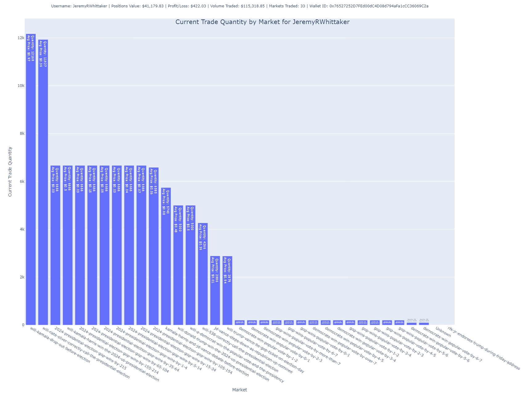
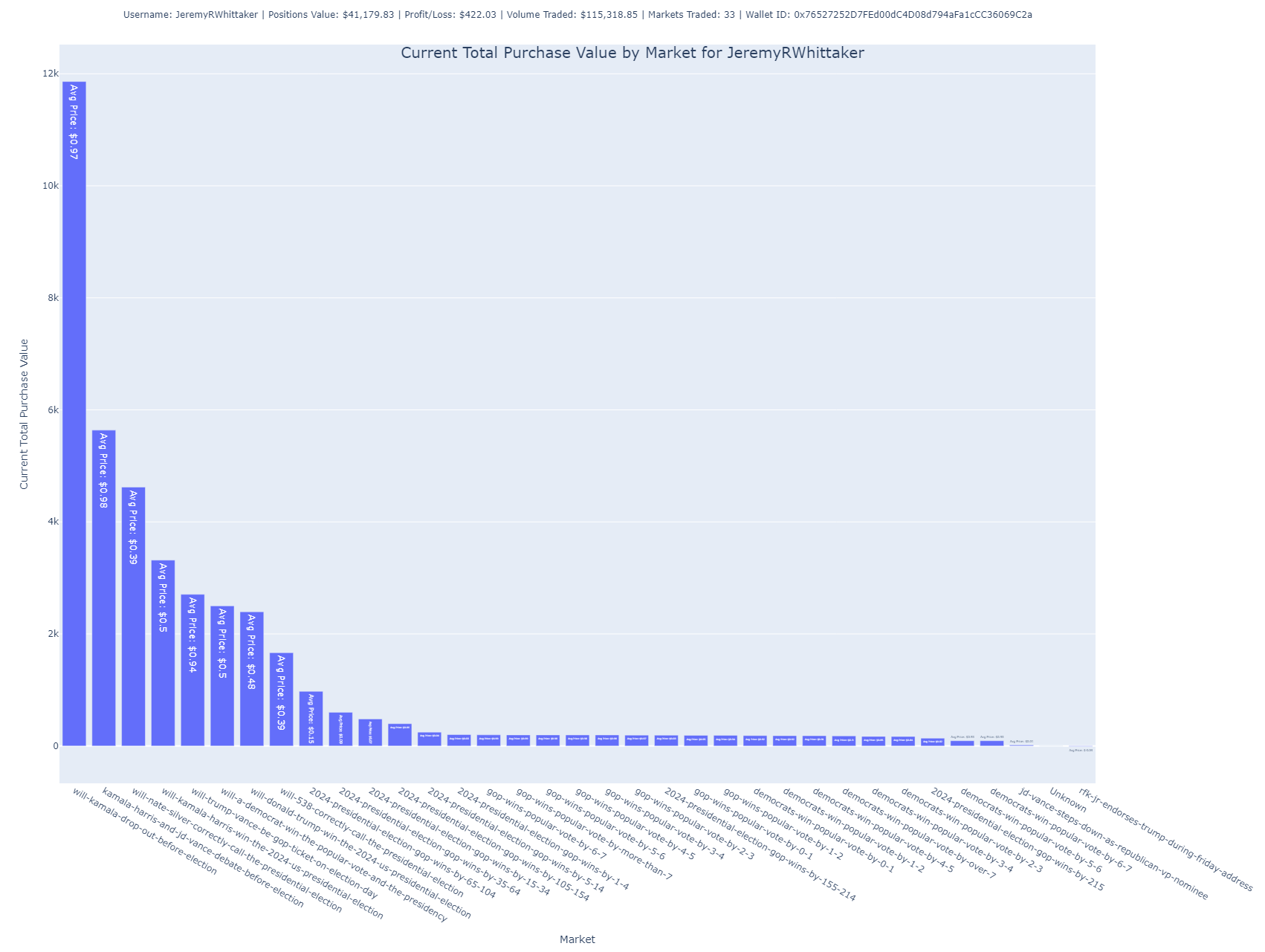


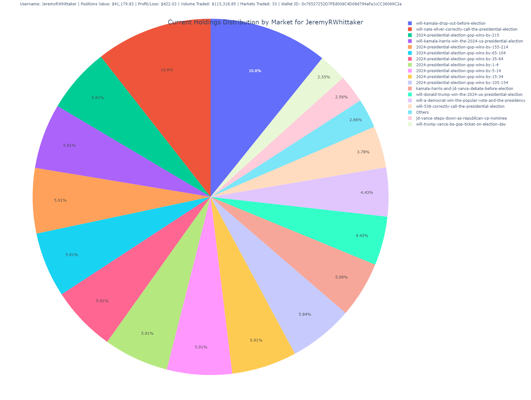

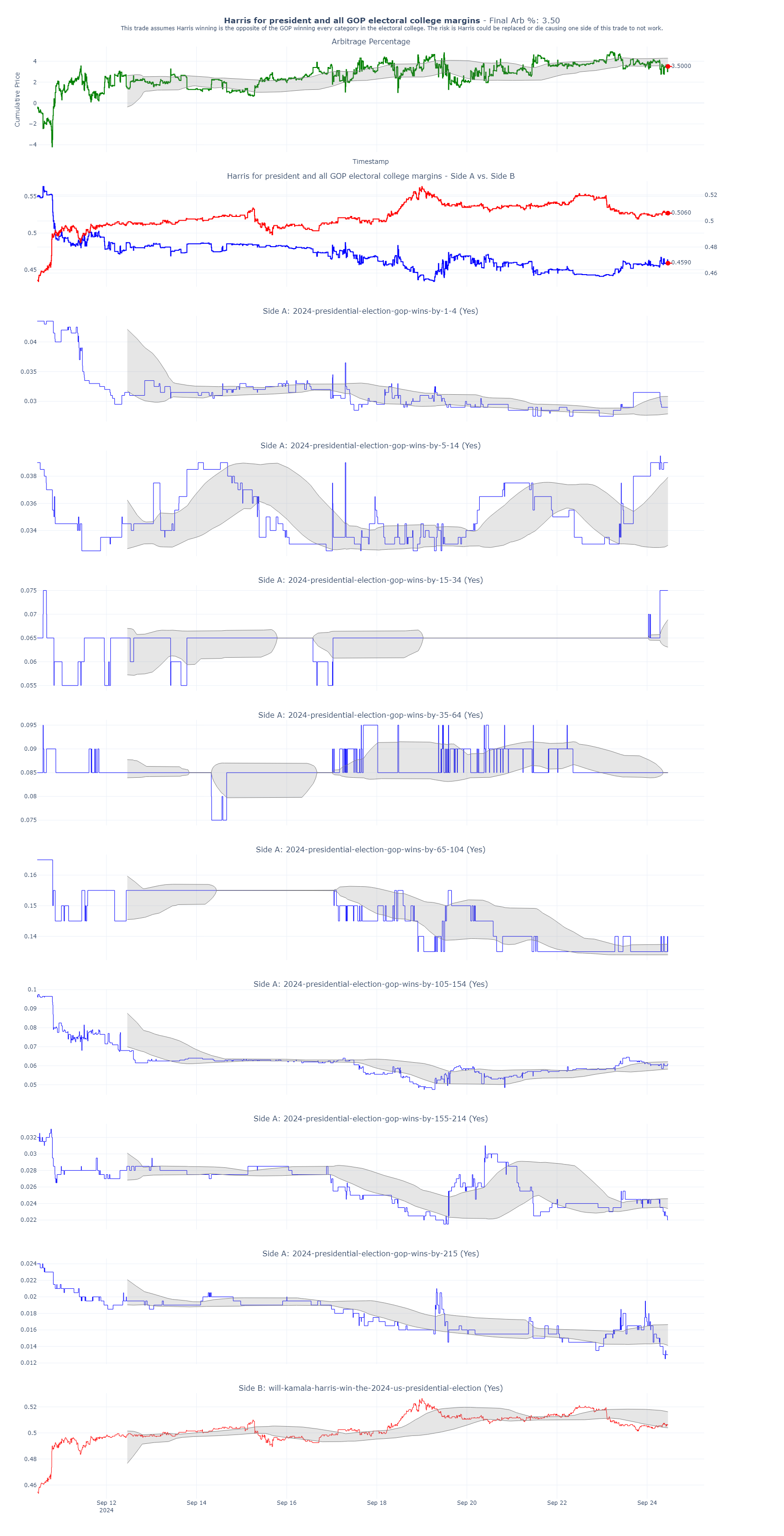

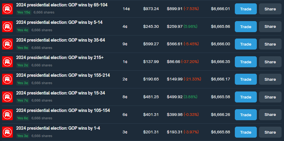
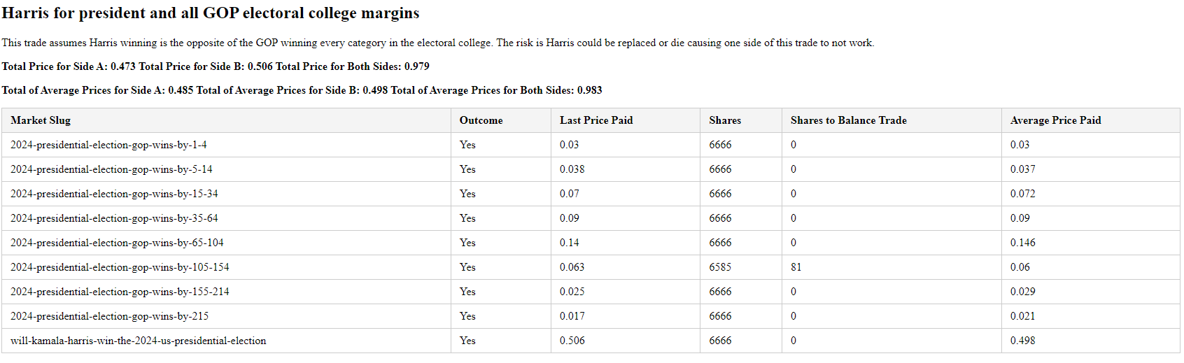
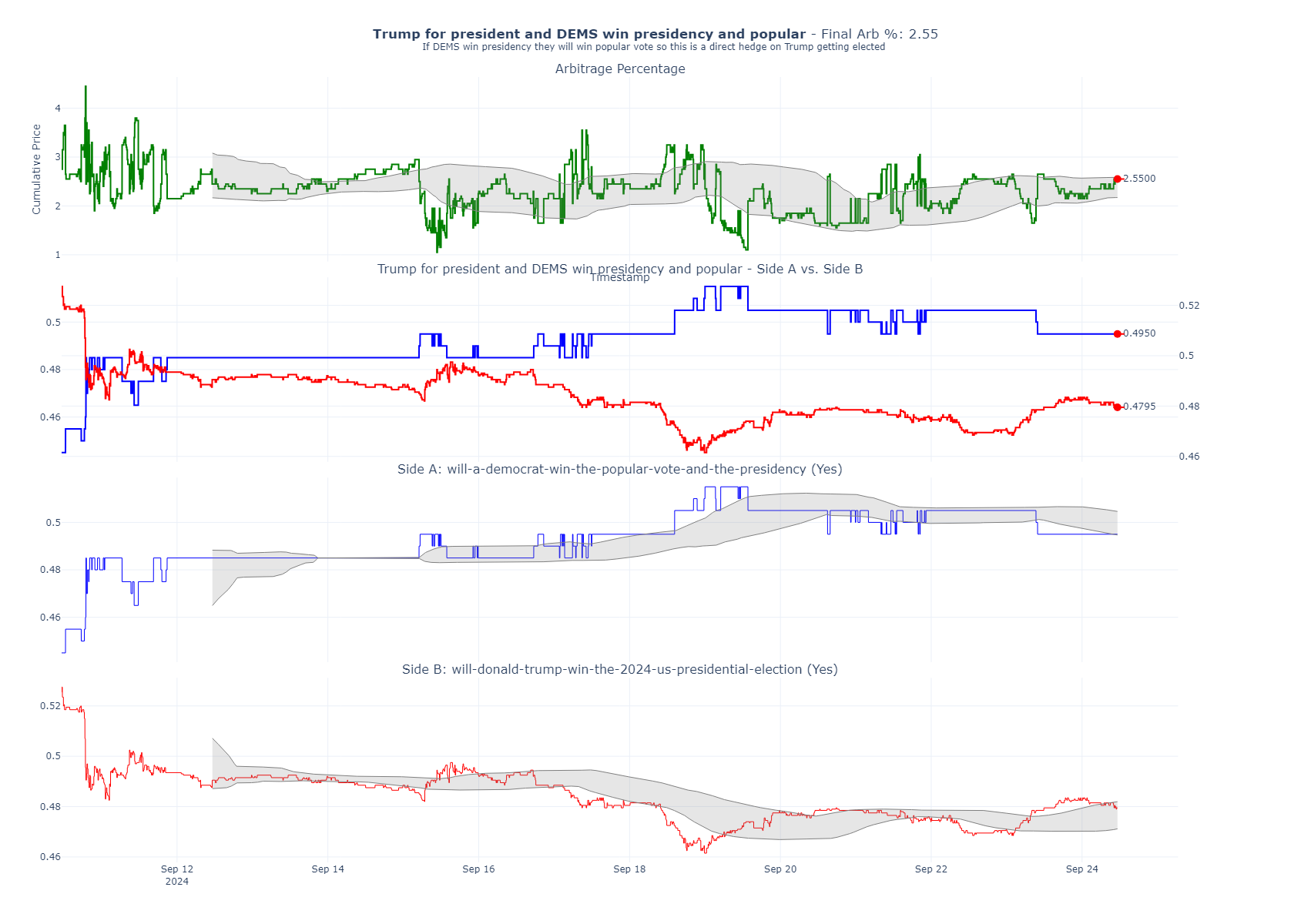

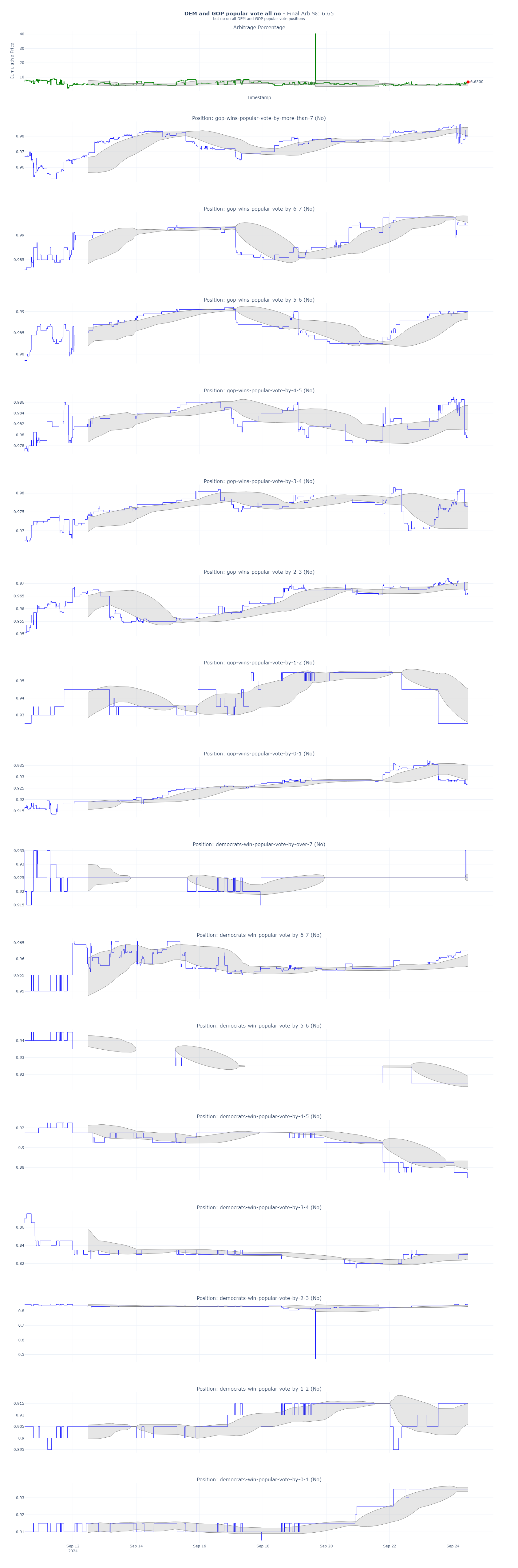
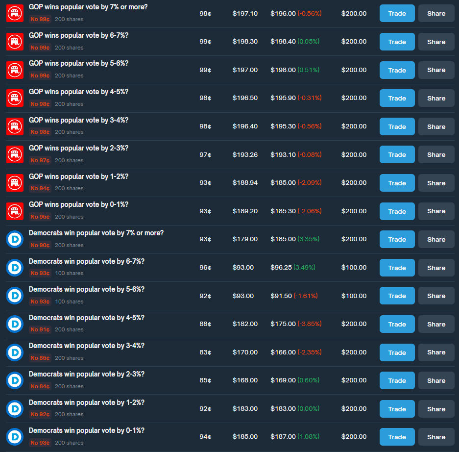


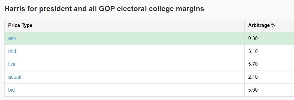
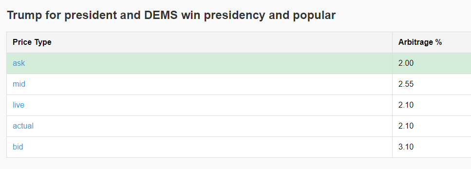
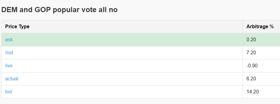
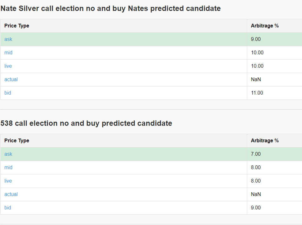
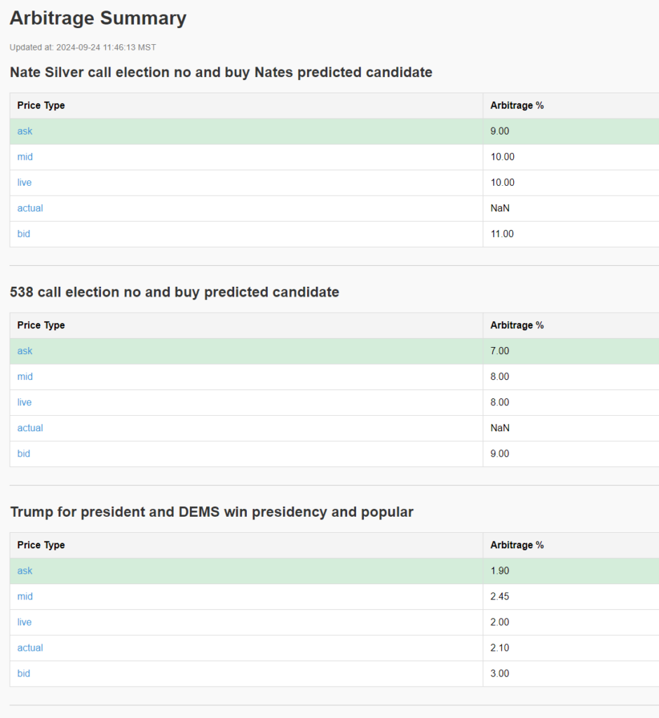


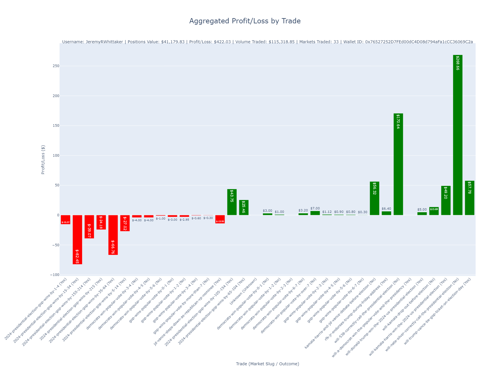
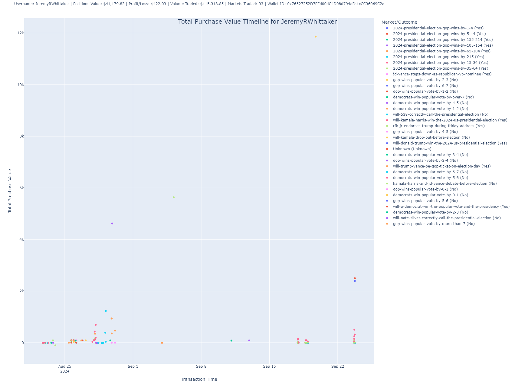


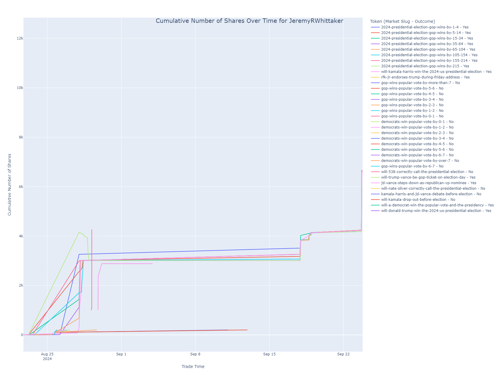
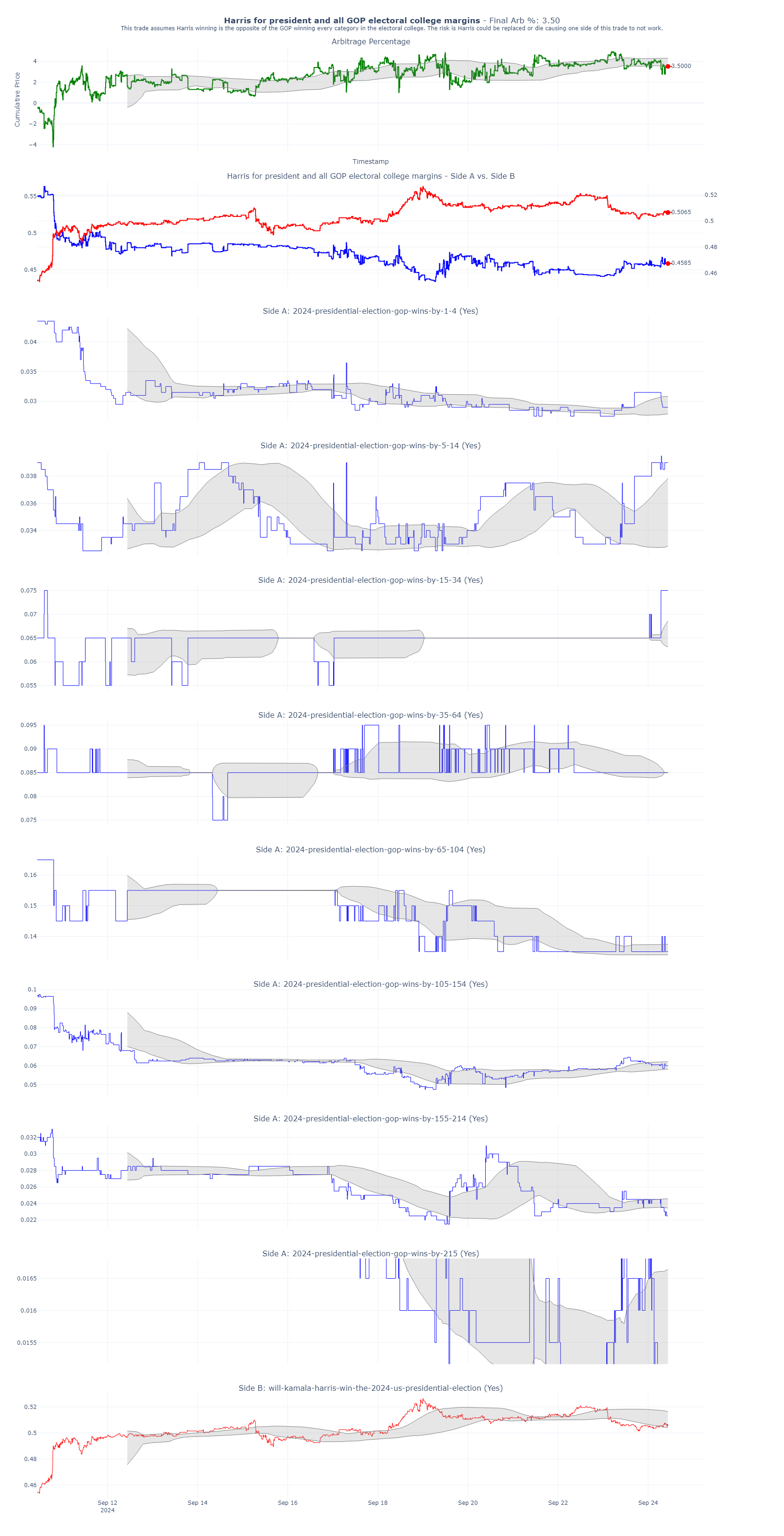
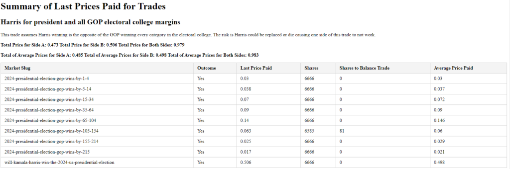
![\[ \text{ROI} = \frac{\text{Profit}}{\text{Total Cost}} \times 100 \]](https://jeremywhittaker.com/wp-content/ql-cache/quicklatex.com-0b2704b9c31db80bf90c952ff7b4a41c_l3.png "Rendered by QuickLaTeX.com")
![\[ \text{ROI} = \frac{102.91}{5637.09} \times 100 = 1.83\% \]](https://jeremywhittaker.com/wp-content/ql-cache/quicklatex.com-bb2e9b748755cac008298c865265b1c0_l3.png "Rendered by QuickLaTeX.com")
![\[ \text{Annual Yield} = \left(1 + \frac{1.83}{100}\right)^{\frac{365}{60}} - 1 \]](https://jeremywhittaker.com/wp-content/ql-cache/quicklatex.com-7d1012ced71b69b8fdeecd3ddb0b2481_l3.png "Rendered by QuickLaTeX.com")
![\[ \text{Annual Yield} \approx 12.09\% \]](https://jeremywhittaker.com/wp-content/ql-cache/quicklatex.com-16c789d2f3dd4ea04923566cd74b7656_l3.png "Rendered by QuickLaTeX.com")