Exploiting Arbitrage – Betting Against Nate Silver for a 54% Yield

I’m always on the hunt for an edge in the markets. After finishing Nate Silver’s book, “On the Edge: The Art of Risking Everything.” this week I thought it would be fitting to write a blog post about an arbitrage opportunity

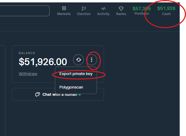
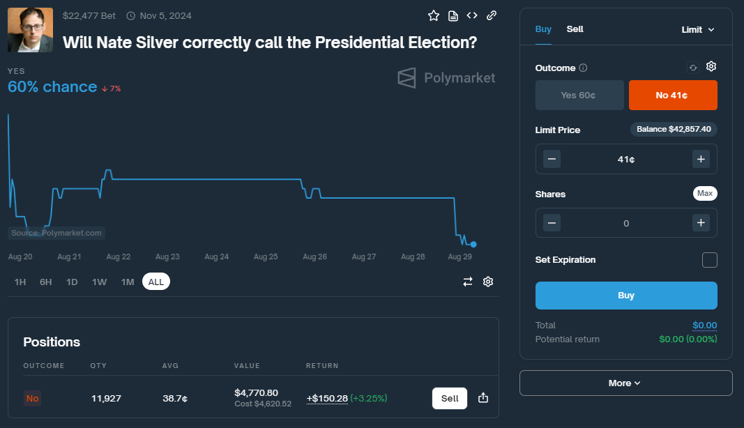
Ironically I’m placing a bet against him on Polymarket.com…. Ok, maybe not technically against him. But earlier today I bought 11,927 ‘No’ shares that he would not call the Presidential election. What’s funny about this position is I think he will accurately call the election. Or at least there is a better than 50/50 chance he will call the election. Making this a bad bet.

You might be wondering why I would do this if I didn’t think it would profit. I will explain how to profit by betting against Nate Silver’s election predictions—a strategy that, if executed correctly, can offer a guaranteed win or at least a break-even outcome, all while potentially yielding a 54% yield on your investment. In this post, I’ll walk you through the mechanics, the math behind it, and how to manage your bets leading up to election day.

The Opportunity: Betting Against Nate Silver


Nate Silver is a well-known figure in election forecasting, and platforms like Polymarket.com allow you to bet on whether he will correctly predict an election outcome. Here’s the edge: you can bet that Nate Silver will be wrong while simultaneously betting on the candidate he predicts to win. If you play it right, this creates a no-risk scenario where you can either break even or secure a small profit with an annualized return of up to 54% (the trade only lasts for 67 days so you won’t actually make 54% this is however the annual yield)

“To succeed in a world full of uncertainty, one must adopt the mindset of the fox, always ready to pivot and re-evaluate when new data presents itself.”

While I might be exploiting a flaw in prediction markets here, Silver’s insights are invaluable for understanding how to think critically about risk and predictions. It’s a reminder that the best strategies are those that remain agile and open to new information.

The Math That Makes It Work

Here’s how it works:

Bet on “NO” for Nate Silver being wrong: Cost C_N = 40 cents.

Bet on the candidate Nate Silver predicts to win: This cost C_C will fluctuate based on the odds, but here’s where it gets interesting.

Conditional Formula

To ensure you either break even or make a profit, here’s the formula to follow:

    \[P =\begin{cases}1 - (C_N + C_C), & \text{if } (C_N + C_C) \leq 1 \\\text{Do not place the bet}, & \text{if } (C_N + C_C) > 1\end{cases}\]

This means:

If C_N + C_C \leq 1: You place the bet, knowing you’ll either break even or profit.

If C_N + C_C > 1: You skip the candidate bet altogether to avoid a loss.

Setting and Managing Your Limit Orders

Nate Silver’s predictions are updated multiple times per week as new data comes in. To optimize this strategy you have to do two things:

  • You have to set a limit order at the inverse of your price that you bought ‘No’ shares for Nate Silver. This will ensure that you break even. C_N + C_C \leq 1
  • As election day moves closer and you are confident that Nate’s predictions are not going to flip you should lock in your profits by buying the candidate that he predicts will win. You must place this trade or you will not be hedged! And if the cost to buy ‘No’ on Nate Silver and the cost of the candidate exceeds 1 you will lose money. C_N + C_C

My Take: A Tight Race Expected

In my opinion, this election is likely to be a close one—a virtual coin toss with odds hovering around 50/50. Given this, the potential profit from this strategy might be around 10%, assuming the market prices stay within a reasonable range. With 67 days left until the election, this profit can be annualized to provide a significant APR.

To calculate the APR, you can use the formula:


    \[\text{APR} = \left( \frac{\text{Profit}}{\text{Investment}} \right) \times \left( \frac{365}{\text{Days until Election}} \right)\]


So, if you’re making about a 10% return over 67 days:

    \[\text{APR} = 0.10 \times \left( \frac{365}{67} \right) \approx 0.54 \text{ or } 54\%\]


Unfortunately, Liquidity is an Issue

As promising as this strategy sounds, there’s one significant drawback: liquidity. I was only able to purchase 11,927 shares of Nate Silver being wrong and 4,266 shares of 538 calling the election for less than 39 cents. Essentially, I bought both trades as they represent the same underlying outcome. This lack of liquidity means that your ability to place large bets or move in and out of positions may be limited, potentially affecting the profitability of this strategy.

Definitions, The Fine Print

One crucial aspect of this strategy that needs to be understood is the timing of Nate Silver’s predictions. Typically, Nate Silver and his team at FiveThirtyEight may continue to update their forecasts until the very last moment—sometimes even until the morning of election day. This means that the candidate Nate predicts to win could change at the last minute, potentially complicating the execution of your bet on the winning candidate.

If Silver’s prediction is “frozen” too late, it may reduce the amount of time you have to place your bet, making it harder to lock in the favorable odds that ensure a profit. Additionally, a last-minute change in prediction could cause significant fluctuations in the betting market, making it difficult to execute your planned hedge. This “fine print” detail is something you should be acutely aware of when executing this strategy, as it could impact your ability to successfully carry out the arbitrage.

In short, while the strategy seems straightforward, the timing of when the prediction is finalized adds a layer of complexity that must be considered to avoid potential pitfalls. It is critical to monitor the forecast updates closely and be prepared to act quickly when the prediction is frozen to maximize the chances of executing the arbitrage successfully.

Is This Actually Arbitrage?

While this strategy appears to be a form of arbitrage, it’s important to recognize that certain unforeseen events could complicate the situation. For example, if one of the candidates were to die before the election, the market dynamics could change dramatically. The sudden withdrawal of a candidate would likely cause a market upheaval, potentially voiding some bets or causing severe losses. This is a reminder that even in what appears to be a “sure thing,” there are always risks that need to be considered. Thus, while this strategy mimics the characteristics of arbitrage, it’s not entirely free of risk.

Conclusion

This arbitrage opportunity isn’t about taking big risks for big rewards. Instead, it’s about leveraging market inefficiencies to guarantee yourself a win, however small. By betting that Nate Silver will be wrong and strategically placing a bet on the candidate he predicts to win, you’re setting yourself up for a situation where the numbers work in your favor—as long as you stick to the math. Just remember, the total cost must not exceed $1. If it does, walk away and wait for the next opportunity.

And if you’re interested in diving deeper into understanding risk and decision-making, I highly recommend Nate Silver’s book “On the Edge: The Art of Risking Everything.” It’s packed with insights on how to think like a fox—adaptable, curious, and always ready to revise your beliefs when new evidence comes to light.

Generating API keys for Polymarket.com

Here is a quick tutorial on how to generate API Key, Secret, and Passphrase to Polymarket.com. This way you can start trading using Python and skip the web interface.

keys.env

The first step is to create an environment file. You only want to populate the PK value. You do not know the other 3 variables yet so just comment them out. You can find this private key by logging in to your Polymarket.com account. Clicking on ‘Cash’, 3 dots, and finally Export Private Key.

#remove the '0x'
PK = "PRIVATE KEY EXPORTED FROM POLYMARKET.COM"

#these are generated through get_api_key.py do not specify these until you run the script with your private key
#API Key: xxxxxxxx-xxxx-xxxxx-xxxx-xxxxxxxxxxxx
#Secret: Lxxxxxxxxxxxxxxxxxxxxxxxxxxxxxxxxxxxxxxxxxx=
#Passphrase: dxxxxxxxxxxxxxxxxxxxxxxxxxxxxxxxxxxxxxxxxxxxxxxxxxxxxxxxxxxxxxe9

generate_api_key.py

import os
from py_clob_client.client import ClobClient
from dotenv import load_dotenv

# Load the environment variables from the specified .env file
load_dotenv('keys.env')

def main():
    host = "https://clob.polymarket.com"
    key = os.getenv("PK")
    chain_id = 137  # Polygon Mainnet chain ID

    # Ensure the private key is loaded correctly
    if not key:
        raise ValueError("Private key not found. Please set PK in the environment variables.")

    # Initialize the client with your private key
    client = ClobClient(host, key=key, chain_id=chain_id)

    # Create or derive API credentials (this is where the API key, secret, and passphrase are generated)
    try:
        api_creds = client.create_or_derive_api_creds()
        print("API Key:", api_creds.api_key)
        print("Secret:", api_creds.api_secret)
        print("Passphrase:", api_creds.api_passphrase)

        # You should now save these securely (e.g., store them in your .env file)
    except Exception as e:
        print("Error creating or deriving API credentials:", e)

if __name__ == "__main__":
    main()

Accessing Polymarket.com Data in Python

Recently I started exploring arbitrage opportunities in the Polymarket.com world. I quickly realized I would need faster access to the data. So I wrote some Python programs to access the platform for data analytics. The documents for doing this are located in the Polymarket docs. Here’s how it works.

Install py-clob-client

pip install py-clob-client<br><br>

Coinbase Wallet

To perform this first block of code you need a Coinbase wallet. Once you have it setup you need to export your private key.

from py_clob_client.client import ClobClient

host = "https://clob.polymarket.com"
private_key = "YOUR_PRIVATE_KEY_GOES_HERE"
chain_id = 137  # Polygon Mainnet

# Initialize the client with private key
client = ClobClient(host, key=private_key, chain_id=chain_id)

api_key_data = client.create_api_key()

print(api_key_data)

Creating keys.py

We can take this outputted data and create our keys.py which will hold our keys.For some reason, the api_passphrase and rename it api_key while commenting out the original api_key. I left the api_secret and original api_passphrase. Now that I have my keys.py I can reference it in my main code


Extracting all of the data

import csv
import json
from py_clob_client.client import ClobClient
from keys import api_key  # Import only the API key
from py_clob_client.clob_types import OpenOrderParams

# Replace with your actual host and chain ID
host = "https://clob.polymarket.com"
chain_id = 137  # Polygon Mainnet

# Initialize the client with only the host, key, and chain_id
client = ClobClient(
    host,
    key=api_key,
    chain_id=chain_id
)

# Initialize variables for pagination
markets_list = []
next_cursor = None

# Fetch all available markets using pagination
while True:
    try:
        # Print the cursor value for debugging
        print(f"Fetching markets with next_cursor: {next_cursor}")

        # Make the API call based on the cursor value
        if next_cursor is None:
            response = client.get_markets()
        else:
            response = client.get_markets(next_cursor=next_cursor)

        # Print the raw response for debugging
        print(f"API Response: {json.dumps(response, indent=2)}")

        # Check if the response is successful and contains data
        if 'data' not in response:
            print("No data found in response.")
            break

        markets_list.extend(response['data'])
        next_cursor = response.get("next_cursor")

        # Exit loop if there's no next_cursor indicating no more data to fetch
        if not next_cursor:
            break

    except Exception as e:
        # Print the exception details for debugging
        print(f"Exception occurred: {e}")
        print(f"Exception details: {e.__class__.__name__}")
        print(f"Error message: {e.args}")
        break

# Debugging step: Print out the raw data to understand its structure
print("Raw Market Data:")
print(json.dumps(markets_list, indent=2))

# Dynamically extract all keys from the markets to create the CSV columns
csv_columns = set()
for market in markets_list:
    csv_columns.update(market.keys())
    # Also include nested keys like tokens
    if 'tokens' in market:
        csv_columns.update({f"token_{key}" for token in market['tokens'] for key in token.keys()})

csv_columns = sorted(csv_columns)  # Sort columns alphabetically for consistency

# Writing to CSV
csv_file = "markets_data.csv"
try:
    with open(csv_file, 'w', newline='') as csvfile:
        writer = csv.DictWriter(csvfile, fieldnames=csv_columns)
        writer.writeheader()
        for market in markets_list:
            row = {}
            for key in csv_columns:
                # Handling nested 'tokens' structure
                if key.startswith("token_"):
                    token_key = key[len("token_"):]
                    row[key] = ', '.join([str(token.get(token_key, 'N/A')) for token in market.get('tokens', [])])
                else:
                    row[key] = market.get(key, 'N/A')
            writer.writerow(row)
    print(f"Data has been written to {csv_file} successfully.")
except IOError as e:
    print(f"Error writing to CSV: {e}")

Output CSV

If all goes as planned you will now have a giant CSV file named markets_data.csv with all the different markets and their values. You can now build on this code to manipulate it to your needs.

Unconventional Success: A Fundamental Approach to Personal Investment by David F. Swensen 

I’ve had Unconventional Success by David F. Swensen on my shelf for five years, but it took me a while to finish. The book is somewhat dense and challenging, yet it offers valuable insights, particularly about the effects of drawdown on a portfolio. Swensen, Yale’s CIO for 36 years, managed to achieve an impressive 12% annual return during his tenure.

One key takeaway is that while the S&P 500 generally outperforms many strategies, certain portfolios can do better overall by minimizing drawdowns. Swensen emphasizes several principles that are common in investment literature:

  1. Equities Should Dominate: Despite being riskier, equities offer higher long-term returns.
  2. Passive Investing Over Active Management: Costs significantly impact your portfolio, so minimize them.
  3. Diversification Is Essential: A portfolio solely composed of equities will suffer from severe drawdowns, which can take years to recover from. A well-balanced portfolio mitigates this risk.
  4. Avoid Market Timing: Base your strategy on long-term thinking.
  5. Rebalancing Is Crucial: Regularly sell overperforming assets and buy underperforming ones.
  6. Consider Tax Implications: Be aware of the tax consequences when buying or selling assets.
  7. Stay Disciplined: Don’t let emotions dictate your investment decisions.

Swensen’s Model Portfolio

Swensen’s recommended allocation includes:

  • U.S. Equities: 30%
  • International Developed Market Equities: 15%
  • Emerging Market Equities: 5%
  • REITs: 20%
  • U.S. Treasury Bonds: 15%
  • TIPS: 15%

Hypothetical Portfolios

I compiled and backtested several hypothetical portfolios based on Swensen’s principles. While most failed to outperform the S&P 500 over a 20-year period, one aggressive portfolio did manage to do so, primarily due to its better handling of drawdowns during the 2008-2009 recession.

Conservative Portfolio: $45,293Conservative B Portfolio: $38,916
Moderate Portfolio: $54,785Moderate B Portfolio: $60,839
Aggressive Portfolio: $64,137Aggressive B Portfolio: $93,856
S&P 500 (SPY): $80,315

Portfolio Allocations

Original Portfolios

  1. Conservative Portfolio:
    • 25% VTI, 10% EFA, 5% VWO, 15% VNQ, 25% IEF, 20% TIP
  2. Moderate Portfolio:
    • 30% VTI, 15% EFA, 10% VWO, 15% VNQ, 15% IEF, 15% TIP
  3. Aggressive Portfolio:
    • 40% VTI, 20% EFA, 15% VWO, 10% VNQ, 10% IEF, 5% TIP

B-Series Portfolios

  1. Conservative B Portfolio:
    • 20% VTSAX, 10% VEA, 5% VWO, 15% VNQ, 25% VBTLX, 25% VIPSX
  2. Moderate B Portfolio:
    • 25% VTSAX, 15% VEA, 10% VWO, 20% VNQ, 15% VBTLX, 15% VIPSX
  3. Aggressive B Portfolio:
    • 35% VTSAX, 20% VEA, 10% VWO, 20% VNQ, 10% VBTLX, 5% VIPSX

Benchmark

  1. S&P 500 (SPY)

While beating the S&P 500 over the long term is challenging, Swensen’s strategies offer a solid foundation for those looking to manage risk and optimize returns. For most investors, simply investing in the S&P 500 might be the best approach, but Swensen shows there are ways to potentially outperform through strategic portfolio management.

Annual Returns (2003 – 2023)

2003

PortfolioReturn
Conservative Portfolio18.34%
Moderate Portfolio19.90%
Aggressive Portfolio21.45%
Conservative B13.39%
Moderate B18.30%
Aggressive B23.95%
S&P 500 (SPY)28.18%

2004

PortfolioReturn
Conservative Portfolio11.55%
Moderate Portfolio12.49%
Aggressive Portfolio14.08%
Conservative B7.42%
Moderate B19.80%
Aggressive B21.28%
S&P 500 (SPY)10.70%

2005

PortfolioReturn
Conservative Portfolio8.62%
Moderate Portfolio10.46%
Aggressive Portfolio12.24%
Conservative B7.57%
Moderate B10.68%
Aggressive B11.77%
S&P 500 (SPY)4.83%

2006

PortfolioReturn
Conservative Portfolio18.71%
Moderate Portfolio21.07%
Aggressive Portfolio23.19%
Conservative B19.47%
Moderate B22.66%
Aggressive B26.71%
S&P 500 (SPY)15.85%

2007

PortfolioReturn
Conservative Portfolio6.92%
Moderate Portfolio7.64%
Aggressive Portfolio9.07%
Conservative B5.04%
Moderate B6.09%
Aggressive B7.82%
S&P 500 (SPY)5.14%

2008

PortfolioReturn
Conservative Portfolio-24.53%
Moderate Portfolio-27.55%
Aggressive Portfolio-31.46%
Conservative B-24.30%
Moderate B-27.57%
Aggressive B-33.20%
S&P 500 (SPY)-36.81%

2009

PortfolioReturn
Conservative Portfolio22.78%
Moderate Portfolio25.46%
Aggressive Portfolio27.59%
Conservative B26.79%
Moderate B33.32%
Aggressive B39.89%
S&P 500 (SPY)26.37%

2010

PortfolioReturn
Conservative Portfolio14.65%
Moderate Portfolio15.73%
Aggressive Portfolio16.57%
Conservative B12.81%
Moderate B18.72%
Aggressive B23.66%
S&P 500 (SPY)15.06%

2011

PortfolioReturn
Conservative Portfolio5.33%
Moderate Portfolio3.66%
Aggressive Portfolio3.92%
Conservative B3.07%
Moderate B4.50%
Aggressive B0.33%
S&P 500 (SPY)1.89%

2012

PortfolioReturn
Conservative Portfolio14.20%
Moderate Portfolio14.95%
Aggressive Portfolio16.05%
Conservative B11.49%
Moderate B13.46%
Aggressive B19.45%
S&P 500 (SPY)15.99%

2013

PortfolioReturn
Conservative Portfolio10.62%
Moderate Portfolio14.34%
Aggressive Portfolio16.07%
Conservative B10.61%
Moderate B12.44%
Aggressive B22.27%
S&P 500 (SPY)32.31%

2014

PortfolioReturn
Conservative Portfolio8.49%
Moderate Portfolio10.03%
Aggressive Portfolio11.11%
Conservative B7.99%
Moderate B11.00%
Aggressive B13.04%
S&P 500 (SPY)13.46%

2015

PortfolioReturn
Conservative Portfolio-1.37%
Moderate Portfolio-2.23%
Aggressive Portfolio-3.02%
Conservative B-1.60%
Moderate B-1.42%
Aggressive B-2.27%
S&P 500 (SPY)1.25%

2016

PortfolioReturn
Conservative Portfolio7.71%
Moderate Portfolio9.56%
Aggressive Portfolio10.96%
Conservative B7.62%
Moderate B8.03%
Aggressive B12.17%
S&P 500 (SPY)12.00%

2017

PortfolioReturn
Conservative Portfolio13.75%
Moderate Portfolio18.11%
Aggressive Portfolio21.11%
Conservative B12.78%
Moderate B17.42%
Aggressive B24.71%
S&P 500 (SPY)21.70%

2018

PortfolioReturn
Conservative Portfolio-6.43%
Moderate Portfolio-8.74%
Aggressive Portfolio-11.04%
Conservative B-6.69%
Moderate B-7.04%
Aggressive B-10.27%
S&P 500 (SPY)-4.56%

2019

PortfolioReturn
Conservative Portfolio21.73%
Moderate Portfolio23.58%
Aggressive Portfolio26.23%
Conservative B19.53%
Moderate B21.70%
Aggressive B29.21%
S&P 500 (SPY)31.22%

2020

PortfolioReturn
Conservative Portfolio10.83%
Moderate Portfolio13.58%
Aggressive Portfolio15.56%
Conservative B10.56%
Moderate B11.04%
Aggressive B14.82%
S&P 500 (SPY)18.37%

2021

PortfolioReturn
Conservative Portfolio12.71%
Moderate Portfolio16.57%
Aggressive Portfolio20.73%
Conservative B14.87%
Moderate B17.24%
Aggressive B23.33%
S&P 500 (SPY)28.75%

2022

PortfolioReturn
Conservative Portfolio-17.25%
Moderate Portfolio-18.32%
Aggressive Portfolio-19.45%
Conservative B-17.07%
Moderate B-17.58%
Aggressive B-19.11%
S&P 500 (SPY)-18.17%

2023

PortfolioReturn
Conservative Portfolio14.22%
Moderate Portfolio15.87%
Aggressive Portfolio17.73%
Conservative B13.49%
Moderate B15.92%
Aggressive B17.73%
S&P 500 (SPY)26.19%

I also created a custom GPT for this book. You can find that here.

Building a DIY Powerwall to offset peak demand cost PT3, install

I finally installed this EG4 battery and inverter to power my house. You can read parts 1 and 2 here if you’re curious why I started this project. I did end up purchasing two batteries instead of one. A single inverter can support up to three batteries per the manufacturer. In my current configuration, I have a 28.6kWh capacity(2 batteries in parallel) which so far appears sufficient to support my house in the peak of July for 3 hours.

Too Small

My first attempt at building this project was with one battery with a 14.3kWh capacity. Remember the original goal was to eliminate all energy from the grid between 3-6 PM when energy is very expensive. You can see below in a couple of examples I was using too much energy and the battery would die. Then I would pull energy from the grid as indicated by that red bar. This was the last week before I installed the second battery.

Just Right

Here is the week after installing the second battery giving me a 28.6kWh capacity.


There is still some red in here when I was testing a few things and the battery was off. Also on the 29th I set the state of charge (SOC) level too low and the battery breaker tripped. EG4 recommends not depleting these any less than 20% SOC. This caused me to lose the battery discharging that entire day as indicated by the 3 red bars.

The EG4 interface was a bit tricky to understand at first. But essentially you just want to configure it to discharge the battery during certain hours and stop with the state of charge gets to a certain level.

The SOC cut-off level can also be configured here.

We can then configure the battery to charge starting at midnight

So essentially all the battery is doing is discharging between 3-6PM and charging at midnight.

Measuring current

This inverter also comes with CT clamps. You stick both of these on each leg of your 220v from your electricity provider. This allows you to monitor the amount of electricity you’re using for your entire house so you don’t back feed any electricity into the grid. You can check these options below to make sure the inverter does not send any electricity upstream.

Cost

Because I had to purchase two batteries and an inverter the cost was a bit more than I anticipated. My total cost for the main components was $11,683.30. I bought it from a local company in Arizona, San Tan Solar. The Residential Clean Energy Credit gives you 30% off the cost bringing the final number to $8,178.31 for 28.6kWh of battery and an inverter. The ultimate goal is to offset all of my energy from 2-8 PM with the solar and the current battery. This is just phase one of a larger project that will include solar. However, now that the inverter is installed I am ready to simply plug in solar panels.

Savings

The savings will be a little difficult to calculate until I’ve generated some usage statistics in my new house. However, below is SRP’s standard rates. We can now switch to the SRP 3-6 program and get all of our energy to about 10c per kWh which is a 30-40% savings. Again, the ultimate goal is to convert this into a solar/battery setup and offset all of our usage from 2-8 PM. This will drastically cut costs as all of our electricity will then be 5c per kWh reducing the cost 60-70% per kWh.