I was doing some analysis of the effects of quantitative easing and asset purchases by the FED. Ran across this data of historical ownership of real estate by wealth percentiles.
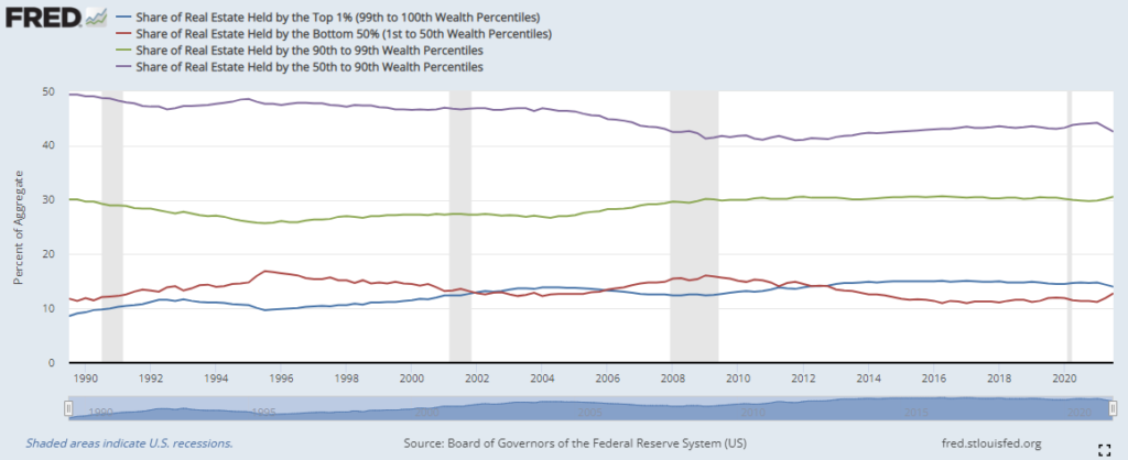

I was doing some analysis of the effects of quantitative easing and asset purchases by the FED. Ran across this data of historical ownership of real estate by wealth percentiles.

If you spend a lot of time analyzing big data then data retrieval is paramount. I’ve written some Python code that I use daily to retrieve data from Federal Reserve Bank of St. Louis and finance.
The first part of this code simply mounts Google drive so you can interface files on your local computer.
working_folder = 'M2 Correlation'

# <----- Make sure to mount drive in Colab first

import os
import sys
if 'google.colab' in str(get_ipython()):
  print('Running on CoLab')
  root_dir='/content/drive/My Drive/Colab Notebooks/' + working_folder
  if os.path.isdir(root_dir):
    %cd $root_dir
  else:
    print('Check your working_folder or if Google drive is mounted')
    sys.exit()
  sys.path.append(root_dir)

  %cd $root_dir

  from IPython.display import clear_output
  clear_output()

  print('Colab code has been executed')
else:
  print('Not running on Colab')
Next, we’re going to install some dependencies.
!pip install yfinance
!pip install pandas-datareader
Next, we’ll import some functions
import yfinance as yf
import pandas_datareader as pdr
import pandas as pd
from datetime import datetime, timedelta
from time import time
from tqdm import tqdm
from pathlib import Path
import plotly.graph_objects as go
import plotly.express as px
import logging
import sys
import matplotlib.pyplot as plt
from datetime import datetime, timedelta
import os
In this next part of our code, we will specify which assets we want data on from FRED and the beginning and end date. Keep in mind some data will not go back as far as you specify. So you’ll have to deal with these blank rows at a later point in the data analysis.
beginning_date = '1900-01-01'
date_today = datetime.now()
end_date = date_today

fred_assets = {
    'cpi_urban_consumers':'CPIAUCSL',
    'gold':'GOLDPMGBD228NLBM',
    'median_house_price':'MSPUS',
    'used_cars':'CUSR0000SETA02',
    'global_all_commodities':'PALLFNFINDEXQ',
    'global_copper':'PCOPPUSDM',
    'spot_crude':'WTISPLC',
    'global_brent_crude':'POILBREUSDM',
    'ground_beef':'APU0000703112',
    'rubber':'PRUBBUSDM',
    'global_raw_materials':'PRAWMINDEXM',
    'global_energy':'PNRGINDEXM',
    'shrimp':'PSHRIUSDM',
    'bacon':'PSHRIUSDM',
    'soybeans':'PSOYBUSDQ',
    'bread':'APU0000702111',
    'propane_tx':'DPROPANEMBTX',
    'global_iron_ore':'PIORECRUSDM',
    'global_wheat':'PWHEAMTUSDM',
    'eggs':'APU0000708111',
    'corn':'PMAIZMTUSDM',
    'global_aluminum':'PALUMUSDM',
    'global_uranium':'PURANUSDM',
    'global_cotton':'PCOTTINDUSDM',
    'us_diesel':'GASDESW',
    'milk':'APU0000709112',
    'global_rice':'PRICENPQUSDM',
    'global_beef':'PBEEFUSDQ',
    'jet_fuel':'DJFUELUSGULF',
    'global_sugar':'PSUGAISAUSDM',
    'coffee':'PCOFFOTMUSDM',
    'global_nickel':'PNICKUSDM',
    'us_gasoline':'APU000074714',
    'global_poultry':'PPOULTUSDM',
    'global_industrial_metals':'PINDUINDEXM',
    'us_flour':'APU0000701111',
    'global_food':'PFOODINDEXM',
    # 'global_fish':'PSALMUSDA', causing issues
    'global_swine':'PPORKUSDM',
    'us_tomatoes':'APU0000712311',
    'lumber':'WPU081',
    'real_median_personal_income':'MEPAINUSA672N',
    'phoenix-mesa-chandler_house_value':'ATNHPIUS38060Q',
    'california_house_value':'CASTHPI',
    'san_francisco_home_price':'SFXRSA',
    '30_year_fixed_mortgage_rates':'MORTGAGE30US',
    'gdp':'GDP',
    'fed_funds_rate':'FEDFUNDS',
    'case-shiller_us_home_index':'CSUSHPINSA',
    'median_household_income':'MEHOINUSA672N',
    'us_house_sales_price':'ASPUS',
    'corporate_bond_yield':'AAA',
    'personal_consumption_expenditures':'PCE',
    'us_industrial_production':'INDPRO',
    'ppi_all_commodities':'PPIACO',
    'us_average_hourly_earnings':'CES0500000003',
    'commercial_industrial_loans':'BUSLOANS',
    'real_disposable_income':'DSPIC96',
    'deposits_all_commercial_banks':'DPSACBW027SBOG',
    'us_home_ownership_rate':'RHORUSQ156N',
    'housing_units_authorized':'PERMIT',
    'coinbase_bitcoin':'CBBTCUSD',
    'loans_leases_bank_credit':'TOTLLNSA',
    'credit_card_delinquency_rate':'DRCCLACBS',
    'disposable_income_per_capita':'A229RX0',
    'personal_income':'PI',
    'poplulation':'POPTHM',
    'global_copper':'PCOPPUSDM',
    'plywood':'WPU083',
    'personal_consumption_expenditures_durable_goods':'PCEDG',
    'gpn':'GNP',
    'total_net_worth_top_1':'WFRBST01134',
    'us_new_one_family_houses':'HSN1F',
    'us_trade_balance':'BOPGSTB',
    'vix':'VIXCLS',
    'yld_10_yr_trsry':'DGS10',


#potential regressors of m2
    'nonfarm_payroll':'PAYEMS',
    'unemployment_rate':'UNRATE',

#potential regressors
    'm2':'M2SL',
    'm3':'MABMM301USM189S',
    'fed_debt':'GFDEBTN',
    'monetary_base':'BOGMBASE',
    'currency_in_circulation':'CURRCIR',
    'm1':'M1SL',
    'real_m2_money_stock':'M2REAL',
    'fed_mbs':'WSHOMCB',
    'fed_total_assets':'WALCL',

          }

yfinance_assets = {

#indices
      'SP 500':'^GSPC',
      'Dow 30':'^DJI',
      'Nasdaq':'^IXIC',
      'NYSE COMPOSITE (DJ)':'^NYA',
      'NYSE AMEX COMPOSITE INDEX':'^XAX',
      'Cboe UK 100':'^BUK100P',
      'Russell 2000':'^RUT',
      'CBOE Volatility Index':'^VIX',
      'FTSE 100':'^FTSE',
      'DAX PERFORMANCE-INDEX':'^GDAXI',
      'CAC 40':'^FCHI',
      'ESTX 50 PR.EUR':'^STOXX50E',
      'Euronext 100 Index':'^N100',
      'BEL 20':'^BFX',
      'MOEX Russia Index':'IMOEX.ME',
      'Nikkei 225':'^N225',
      'HANG SENG INDEX':'^HSI',
      'SSE Composite Index':'000001.SS',
      'Shenzhen Component':'399001.SZ',
      'STI Index':'^STI',
      'SP ASX 200':'^AXJO',
      'ALL ORDINARIES':'^AORD',
      'SP BSE SENSEX':'^BSESN',
      'Jakarta Composite Index':'^JKSE',
      'FTSE Bursa Malaysia KLCI':'^KLSE',
      'SP NZX 50 INDEX GROSS':'^NZ50',
      'KOSPI Composite Index':'^KS11',
      'TSEC weighted index':'^TWII',
      'SP TSX Composite index':'^GSPTSE',
      'IBOVESPA':'^BVSP',
      'IPC MEXICO':'^MXX',
      'SP CLX IPSA':'^IPSA',
      'MERVAL':'^MERV',
      'TA-125':'^TA125.TA',
      'EGX 30 Price Return Index':'^CASE30',
      'Top 40 USD Net TRI Index':'^JN0U.JO',

#currency
      'EURUSD':'EURUSD=X',
      'USDJPY':'JPY=X',
      'GBPUSD':'GBPUSD=X',
      'AUDUSD':'AUDUSD=X',
      'NZDUSD':'NZDUSD=X',
      'EURJPY':'EURJPY=X',
      'GBPJPY':'GBPJPY=X',
      'EURGBP':'EURGBP=X',
      'EURCAD':'EURCAD=X',
      'EURSEK':'EURSEK=X',
      'EURCHF':'EURCHF=X',
      'EURHUF':'EURHUF=X',
      'EURJPY':'EURJPY=X',
      'USDCNY':'CNY=X',
      'USDHKD':'HKD=X',
      'USDSGD':'SGD=X',
      'USDINR':'INR=X',
      'USDMXN':'MXN=X',
      'USDPHP':'PHP=X',
      'USDIDR':'IDR=X',
      'USDTHB':'THB=X',
      'USDMYR':'MYR=X',
      'USDZAR':'ZAR=X',
      'USDRUB':'RUB=X',


#futures
      '10-Year T-Note Futures,Mar-2022':'ZN=F',
      'E-Mini SP 500 Mar 22':'ES=F',
      'Five-Year US Treasury Note Futu':'ZF=F',
      'Nasdaq 100 Mar 22':'NQ=F',
      'Crude Oil':'CL=F',
      '2-Year T-Note Futures,Mar-2022':'ZT=F',
      'U.S. Treasury Bond Futures,Mar-':'ZB=F',
      'Natural Gas Mar 22':'NG=F',
      'E-mini Russell 2000 Index Futur':'RTY=F',
      'Mini Dow Jones Indus.-$5 Mar 22':'YM=F',
      'Corn Futures,May-2022':'ZC=F',
      'Gold':'GC=F',
      'Sugar #11 May 22':'SB=F',
      'Soybean Futures,May-2022':'ZS=F',
      'Copper Mar 22':'HG=F',
      'RBOB Gasoline Mar 22':'RB=F',
      'Heating Oil Mar 22':'HO=F',
      'Silver':'SI=F',
      'Soybean Oil Futures,May-2022':'ZL=F',
      'Brent Crude Oil Last Day Financ':'BZ=F',
      'Soybean Meal Futures,May-2022':'ZM=F',
      'Micro Gold Futures,Apr-2022':'MGC=F',
      'Cocoa May 22':'CC=F',
      'KC HRW Wheat Futures,Mar-2022':'KE=F',
      'Coffee May 22':'KC=F',
      'Lean Hogs Futures,Apr-2022':'HE=F',
      'Cotton May 22':'CT=F',
      'Platinum Apr 22':'PL=F',
      'Live Cattle Futures,Apr-2022':'LE=F',
      'Feeder Cattle Futures,Mar-2022':'GF=F',
      'Micro Silver Futures,Mar-2022':'SIL=F',
      'Palladium Mar 22':'PA=F',
      'Orange Juice May 22':'OJ=F',
      'Rough Rice Futures,May-2022':'ZR=F',
      'Oat Futures,May-2022':'ZO=F',
      'Random Length Lumber Futures':'LBS=F',
      'Mont Belvieu LDH Propane (OPIS)':'B0=F',


# #etf
      'SPDR SP 500 ETF Trust':'SPY',
      'iShares Core SP 500 ETF':'IVV',
      'Vanguard Total Stock Market ETF':'VTI',
      'Vanguard SP 500 ETF':'VOO',
      'Invesco QQQ Trust':'QQQ',
      'Vanguard FTSE Developed Markets ETF':'VEA',
      'iShares Core MSCI EAFE ETF':'IEFA',
      'Vanguard Value ETF':'VTV',
      'iShares Core U.S. Aggregate Bond ETF':'AGG',
      'Vanguard Total Bond Market ETF':'BND',
      'Vanguard FTSE Emerging Markets ETF':'VWO',
      'Vanguard Growth ETF':'VUG',
      'iShares Core MSCI Emerging Markets ETF':'IEMG',
      'iShares Core SP Small-Cap ETF':'IJR',
      'iShares Russell 1000 Growth ETF':'IWF',
      'Vanguard Dividend Appreciation ETF':'VIG',
      'iShares Core SP Mid-Cap ETF':'IJH',
      'iShares Russell 2000 ETF':'IWM',
      'SPDR Gold Shares':'GLD',
      'iShares Russell 1000 Value ETF':'IWD',
      'iShares MSCI EAFE ETF':'EFA',
      'Vanguard Total International Stock ETF':'VXUS',
      'Vanguard Mid-Cap ETF':'VO',
      'Vanguard Information Technology ETF':'VGT',
      'Financial Select Sector SPDR Fund':'XLF',
      'Vanguard Total International Bond ETF':'BNDX',
      'Vanguard Intermediate-Term Corporate Bond ETF':'VCIT',
      'Vanguard Real Estate ETF':'VNQ',
      'Technology Select Sector SPDR Fund':'XLK',
      'Vanguard Small Cap ETF':'VB',
      'iShares Core SP Total U.S. Stock Market ETF':'ITOT',
      'Vanguard High Dividend Yield Index ETF':'VYM',
      'Vanguard Short-Term Bond ETF':'BSV',
      'Vanguard Short-Term Corporate Bond ETF':'VCSH',
      'iShares TIPS Bond ETF':'TIP',
      'iShares iBoxx $ Investment Grade Corporate Bond ETF':'LQD',
      'Vanguard FTSE All-World ex-US Index Fund':'VEU',
      'iShares SP 500 Growth ETF':'IVW',
      'Health Care Select Sector SPDR Fund':'XLV',
      'Energy Select Sector SPDR Fund':'XLE',
      'Schwab U.S. Large-Cap ETF':'SCHX',
      'Schwab US Dividend Equity ETF':'SCHD',
      'Invesco SP 500® Equal Weight ETF':'RSP',
      'iShares Core MSCI Total International Stock ETF':'IXUS',
      'SPDR Dow Jones Industrial Average ETF Trust':'DIA',
      'iShares Russell 1000 ETF':'IWB',
      'iShares Gold Trust':'IAU',
      'iShares MSCI Emerging Markets ETF':'EEM',
      'iShares Russell Midcap ETF':'IWR',
      'Schwab International Equity ETF':'SCHF',
      'iShares MSCI USA Min Vol Factor ETF':'USMV',
      'Vanguard Large Cap ETF':'VV',
      'Vanguard Small Cap Value ETF':'VBR',
      'iShares National Muni Bond ETF':'MUB',
      'iShares MBS ETF':'MBB',
      'Vanguard Total World Stock ETF':'VT',
      'iShares SP 500 Value ETF':'IVE',
      'iShares ESG Aware MSCI USA ETF':'ESGU',
      'iShares 1-5 Year Investment Grade Corporate Bond ETF':'IGSB',
      'iShares Core Dividend Growth ETF':'DGRO',
      'iShares MSCI USA Quality Factor ETF':'QUAL',
      'Schwab U.S. Broad Market ETF':'SCHB',
      'Vanguard FTSE Europe ETF':'VGK',
      'iShares 1-3 Year Treasury Bond ETF':'SHY',
      'Schwab U.S. TIPS ETF':'SCHP',
      'SPDR SP Dividend ETF':'SDY',
      'iShares Select Dividend ETF':'DVY',
      'Consumer Discretionary Select Sector SPDR Fund':'XLY',
      'Vanguard Short-Term Inflation-Protected Securities ETF':'VTIP',
      'SPDR SP Midcap 400 ETF Trust':'MDY',
      'iShares Preferred Income Securities ETF':'PFF',
      'ProShares UltraPro QQQ':'TQQQ',
      'iShares J.P. Morgan USD Emerging Markets Bond ETF':'EMB',
      'JPMorgan Ultra-Short Income ETF':'JPST',
      'iShares iBoxx $ High Yield Corporate Bond ETF':'HYG',
      'iShares MSCI ACWI ETF':'ACWI',
      'Industrial Select Sector SPDR Fund':'XLI',
      'iShares 7-10 Year Treasury Bond ETF':'IEF',
      'iShares Core Total USD Bond Market ETF':'IUSB',
      'iShares MSCI EAFE Value ETF':'EFV',
      'iShares U.S. Treasury Bond ETF':'GOVT',
      'Vanguard Health Care ETF':'VHT',
      'Vanguard Mid-Cap Value ETF':'VOE',
      'iShares 20+ Year Treasury Bond ETF':'TLT',
      'Schwab U.S. Small-Cap ETF':'SCHA',
      'Schwab U.S. Large-Cap Growth ETF':'SCHG',
      'iShares MSCI USA Value Factor ETF':'VLUE',
      'Vanguard Mortgage-Backed Securities ETF':'VMBS',
      'Vanguard Extended Market ETF':'VXF',
      'iShares Russell 2000 Value ETF':'IWN',
      'Consumer Staples Select Sector SPDR Fund':'XLP',
      'Vanguard Tax-Exempt Bond ETF':'VTEB',
      'iShares Russell Mid-Cap Value ETF':'IWS',
      'SPDR Bloomberg 1-3 Month T-Bill ETF':'BIL',
      'Dimensional U.S. Core Equity 2 ETF':'DFAC',
      'iShares MSCI EAFE Small-Cap ETF':'SCZ',
      'Vanguard Intermediate-Term Bond ETF':'BIV',
      'Vanguard Short-Term Treasury ETF':'VGSH',
      'Vanguard Small Cap Growth ETF':'VBK',
      'iShares Short Treasury Bond ETF':'SHV',


# stocks
      'Berkshire Hathaway':'brk-a',
      'Johnson and Johnson':'jnj',
      'abnb':'abnb',
      'adbe':'adbe',
      'crwd':'crwd',
      'dis':'dis',
      'fvrr':'fvrr',
      'gm':'gm',
      'msft':'msft',
      'shop':'shop',
      'spot':'spot',
          }
Retrieving code from yfinance is slightly different so we’ll specify those assets next. You can download almost any stock, index, or ETF you want from Yahoo Finance.
yfinance_assets = {

#index
    'spy500':'^gspc',
    'nasdaq':'^IXIC',
    'nasdaq_100':'^NDX',
    'djia':'^DJI',
    'wilshire5000':'^W5000',
    'nasdaq':'^IXIC',
    'russell_2000':'^RUT',


# #etf
      'etf_djia':'DIA', #mega
      'etf_large_cap':'SPY', #large cap
      'etf_mid_cap':'IJH', #mid cap
      'etf_small_cap':'IWO', #small cap
      'etf_mall_cap_value':'VBR', #small cap value
      'etf_small_cap_growth':'VBK', #small cap growth
      'etf_micro_cap':'IWM', #micro cap
      'etf_emerging_markets':'VEIEX', #emerging markets
      'etf_reit':'IYR', #reit
      'etf_high_yield_bonds':'HYG', #high yield bonds
      'etf_investment_grade_bonds':'LQD', #investment grade bonds
      'etf_gld':'GLD', #gold etf
      'etf_nasdaq':'QQQ', #nasdaq etf
      'etf_total_market':'VTI', #etf total market

          }
I don’t like downloading all my data every day. So this function I wrote backs up your dataframe.
def save_df(temp_df, filename):
  pd.to_pickle(df,f'{filename}.pkl')
  temp_df.to_csv(f'{filename}.csv')
This section of code will not only plot the asset so you can visually diagnose it but it will save it to your Google drive in a subfolder.
def plot_and_save(df_temp,folder_name):
  for col in df_temp.columns:
    df_temp2 = pd.DataFrame()
    df_temp2 = df_temp[f'{col}']
    df_temp2.dropna(axis='rows', inplace=True)
    fig = px.line(df_temp2, x=df_temp2.index, y=f'{col}', color_discrete_sequence=['red'])
    try:
      fig.write_html(f'{folder_name}/{col}.html')
    except:
      os.makedirs(f'{folder_name}')
      fig.write_html(f'{folder_name}/{col}.html')
    #comment out to save memory
    fig.show()
Here’s the code to retrieve all your FRED data.
def get_fred_prices(assets):
  df_temp = pd.DataFrame(index=pd.date_range(start=beginning_date,end=end_date,freq='D'))
  # df_yearly = pd.DataFrame(index=pd.date_range(start=beginning_date,end=end_date,freq='A'))
  for key, value in assets.items():
    print('Getting {} with symbol {}'.format(key, value))
    try:
      df_temp[f'{key}'] = pdr.DataReader(f'{value}','fred',beginning_date,date_today)
    except:
      print('Error getting {}'.format(value))
    df_temp.ffill(inplace=True)
  return(df_temp)
Here is the code to retrieve all your yfinance data.
def get_yfinance_prices(assets):
  df_temp = pd.DataFrame(index=pd.date_range(start=beginning_date,end=end_date,freq='D'))
  for key, value in assets.items():
    print('Getting {} with symbol {}'.format(key, value))
    try:
      df_temp[f'{key}'] = yf.download(f'{value}',beginning_date,date_today,progress=True).drop(columns=['Open','High','Low','Close','Volume'])
    except:
      print('Error getting {}'.format(value))
    df_temp.ffill(inplace=True)
  return(df_temp)
And finally, a function to bring all your data together.
def get_asset_prices(filename):
  df_fred = get_fred_prices(fred_assets)
  df_yfinance = get_yfinance_prices(yfinance_assets)
  df = pd.concat([df_fred, df_yfinance], axis=1)
  return(df)
This is the code that will actually retrieve your data. It will also drop all the lines that are completely blank. Then it saves the dataframe and proceeds with plotting the data
df = get_asset_prices('asset_prices')
df.dropna(how='all', inplace=True)
save_df(df, 'asset_prices')
df = pd.read_pickle("asset_prices.pkl")
plot_and_save(df,'asset_prices')
Here is a sample of one of the downloads:
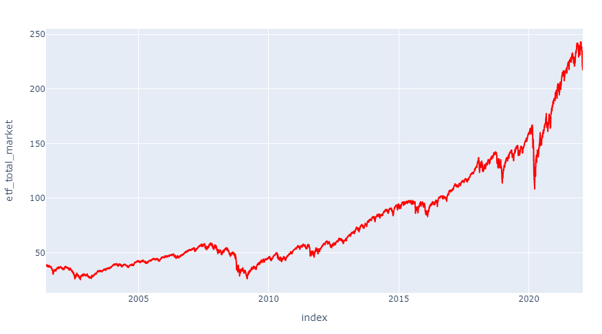
Now that we’ve downloaded the data we want a visualization of the data so we can see chunks of missing data. missingno is a great tool for that. Keep in mind I forward filled the assets in a previous function. What this means is that if the stock market closes on Friday it will show the price of the asset to be the same on Saturday and Sunday.
So think of this chart below as the left being today and the right being 1900. You can see some data from these sources is only available for short time frames, shorter the bar. In this example, you can see there is complete data for producer price index for commodities.
import missingno as msno
msno.bar(df)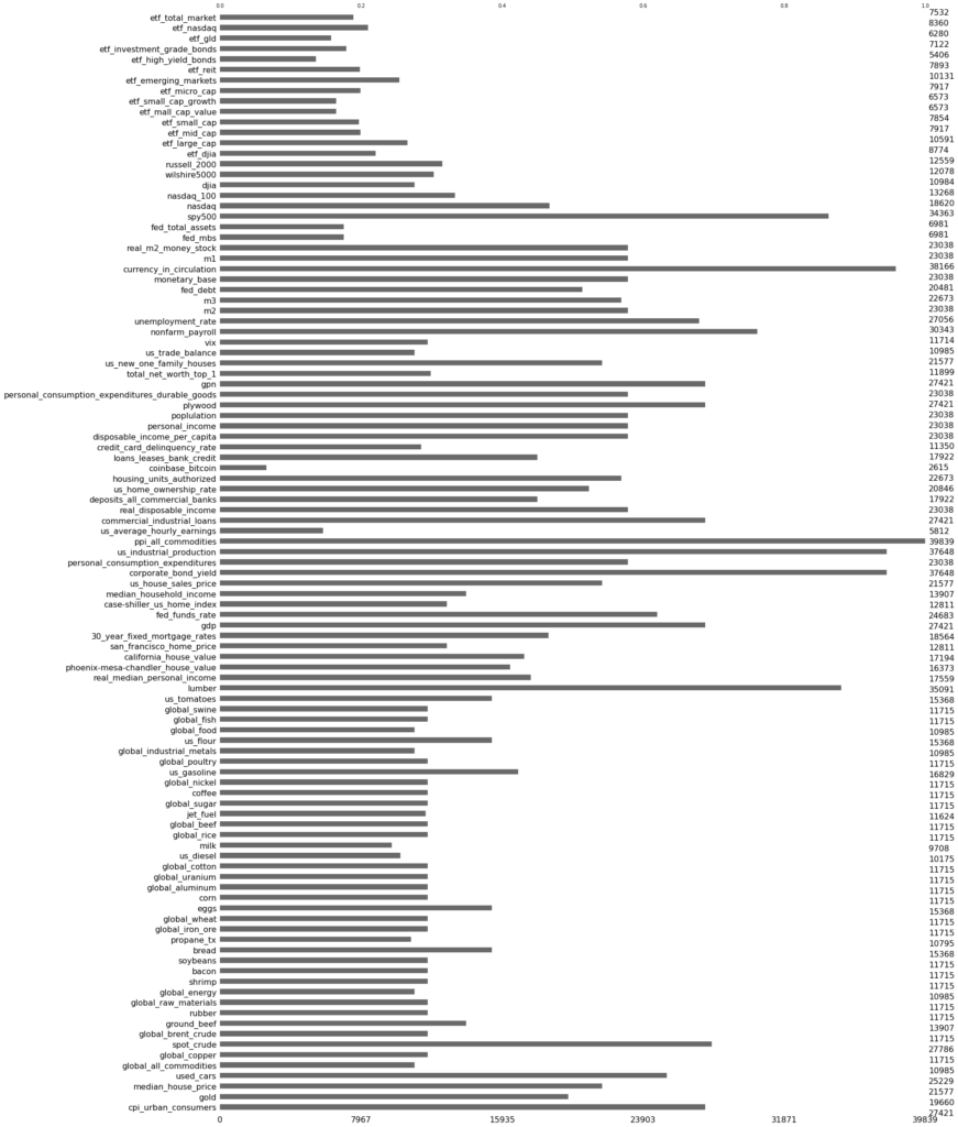
Let’s take a quick look at the first few rows of the data below. You can see most of the data from 1913 is NaN. This means it doesn’t exist in your dataframe. I will talk about cutting out this data later so you don’t have a bunch of empty datasets.
df.head()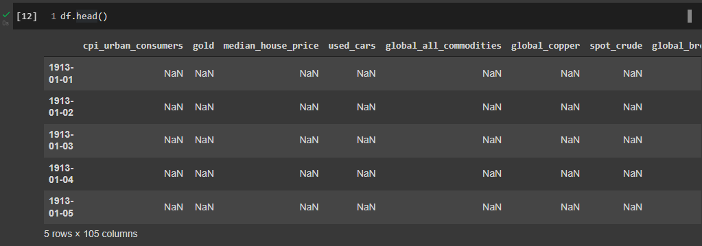
And finally, we’ll look at the information of the dataframe
df.info()
That’s it you’ve downloaded your asset prices and they are all contained in one dataframe and ready for further modification and analysis.
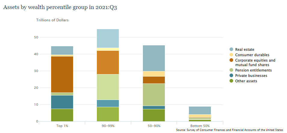
I’m sitting here doing some completely unrelated research and I stumbled across this figure which I’ve seen multiple times in the past. It has always surprised me. As the markets become extremely volatile this month I wonder, what is the impact on the bottom 50% of Americans? If you look at this chart it barely even registers when stacked with other assets. Real estate is their primary asset.
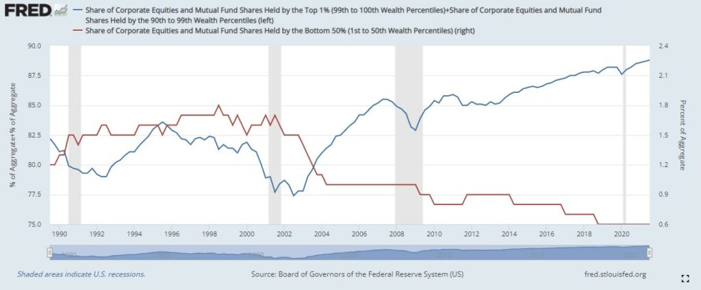
What’s interesting is if you look at this breakdown by percentile historically. The top 10% own 89% of all equities. While the entire bottom 50% own just .6%.
Now let’s take a look at the top 50% vs. the bottom 50%. We already know the bottom 50% of Americans own just .6% of equities. The top 50% own 99.4% of the balance of equities.
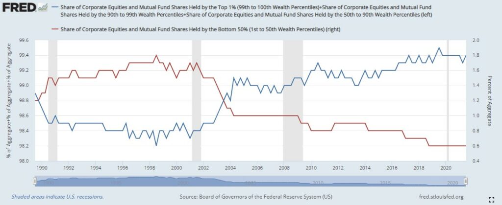
If you’re looking for the source of political turmoil in our country I don’t think we need to look much further than the wealth gap. Half of our population has no vested interest in corporations in America. I can’t imagine turmoil subsides any time soon for our country until we address the wealth gap.
I was recently chatting with a buddy about investing in real estate or stocks and which was better. I decided to use Python to analyze what that investment would look like. I used data from FRED and yfinance which is one of my favorite sources for historical data. Although they do not offer smaller timeframes.

The first thing I’m going to do is set the dates I’m interested in.
beginning_date = '1900-01-01'
date_today = datetime.now()
end_date = date_today
I’m not going to use FRED and YFinance which are two Python plugins to download historical data.
df = yf.download('^gspc',beginning_date,date_today,progress=True).drop(columns=['Open','High','Low','Close','Volume']).rename(columns={'Adj Close':'SP500'})
df = df.rename(columns={'Adj Close':'SP500'})

df['MSPUS'] = pdr.DataReader('MSPUS','fred',beginning_date,date_today)
df = df.rename(columns={'MSPUS':'Median_House_price'})
The stock market index symbol from Yahoo is ^gspc as you can see in the code above. The median house price is MSPUS from FRED.
df = df.ffill(axis=0)

df['Median_House_price_pct_change'] = df['Median_House_price'].pct_change()*100
df['SP500_pct_change'] = df['SP500'].pct_change()*100
df = df.dropna()

df['Median_House_price_pct_change_cumsum'] = df['Median_House_price_pct_change'].cumsum()
df['SP500_pct_change_cumsum'] = df['SP500_pct_change'].cumsum()
df = df.dropna()

df['spread'] = df['SP500_pct_change_cumsum'].sub(df['Median_House_price_pct_change_cumsum'])


df.tail(20)
The Median house price data is quarterly so I’m using ffill to forward fill the data.
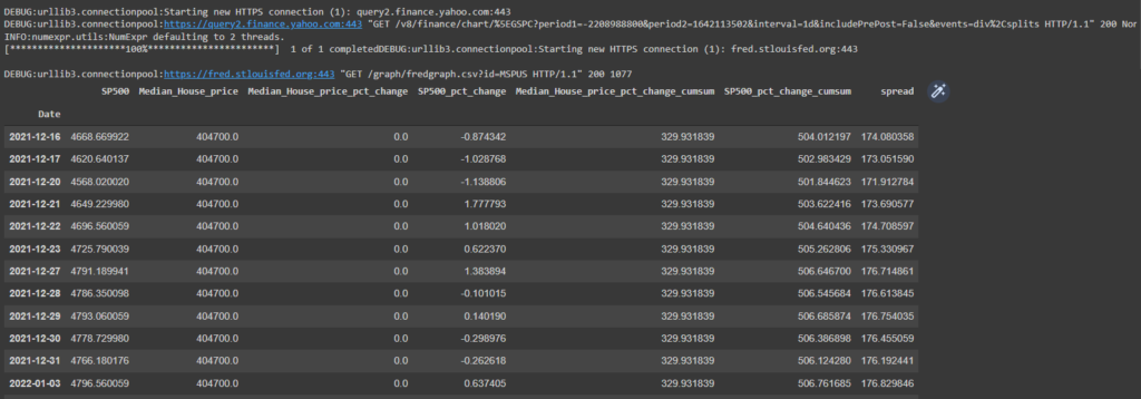
What I’m essentially doing next is creating columns in my DataFrame for the following:
My DataFrame now looks like this.
If I plot the cumulative sum I get this.
fig1 = px.line(df, x=df.index, y='Median_House_price_pct_change_cumsum', color_discrete_sequence=['red'])
fig2 = px.line(df, x=df.index, y='SP500_pct_change_cumsum', color_discrete_sequence=['blue'])

fig3 = go.Figure(data=fig1.data + fig2.data)
fig3.show()
This shows stocks overall since 1963 have outperformed housing.
  fig1 = px.line(df, x=df.index, y='spread', color_discrete_sequence=['red'])
  fig1.show()
This code actually plots the spread between the two assets.

Now I’m going to create some more columns in my DataFrame
df_annual=pd.DataFrame()
df_annual['SP500_pct_change'] = df['SP500_pct_change'].resample('1A').sum()
df_annual['Median_House_price_pct_change'] = df['Median_House_price_pct_change'].resample('1A').sum()
df_annual['SP500_pct_change_cumsum'] = df_annual['SP500_pct_change'].cumsum()
df_annual['Median_House_price_pct_change_cumsum'] =  df_annual['Median_House_price_pct_change'].cumsum()
df_annual.dropna(inplace=True)
df_annual['YoY_spread'] = df_annual['SP500_pct_change'].sub(df_annual['Median_House_price_pct_change'])
df_annual['cumulative_spread'] = df_annual['SP500_pct_change_cumsum'].sub(df_annual['Median_House_price_pct_change_cumsum'])

df_annual.drop(df_annual.index[-1],inplace=True)
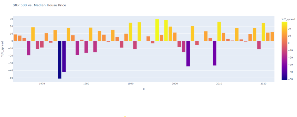
What I’m doing here is resampling my data to annual as it is broken down currently by quarter. The main difference in this code is I’m computing an annual year-over-year return of S&P 500 vs. median house price in the United States. Here is the new DataFrame header.

I’m going to replot this data using the annualized data. Should be almost identical to my first chart.
fig1 = px.line(df_annual, x=df_annual.index, y='Median_House_price_pct_change_cumsum', color_discrete_sequence=['red'])
fig2 = px.line(df_annual, x=df_annual.index, y='SP500_pct_change_cumsum', color_discrete_sequence=['blue'])

fig3 = go.Figure(data=fig1.data + fig2.data)
fig3.show()

And finally, I’m computing the annualized year-over-year spread between S&P 500 and median housing prices. This gives a better idea of the annual returns as opposed to the cumulative returns. Where the bar graph is above 0 indicates the stock market outperformed real estate that year. If the bar is below 0 that indicates the real estate market outperformed the stock market.
And finally the cumulative spread.

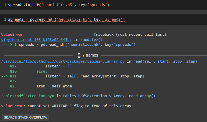
If you’re getting this error when trying to read a simple .h5 file. Change your code when you originally create the .h5 file to specify format=’table’ This should resolve the issue.
