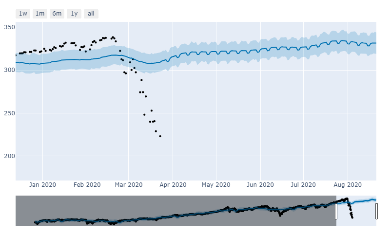
When analyzing historical time frame data in machine learning it needs to be normalized. In this code example, I will show how to get S&P data then convert it to a percent of daily increase/decrease as well as a logarithmic daily increase/decrease.
The first part of this code will use yfinance as our datasource.
#we're going to use yfinance as our data source
!pip install yfinance --upgrade --no-cache-dir

import pandas as pd
import numpy as np
import yfinance as yf
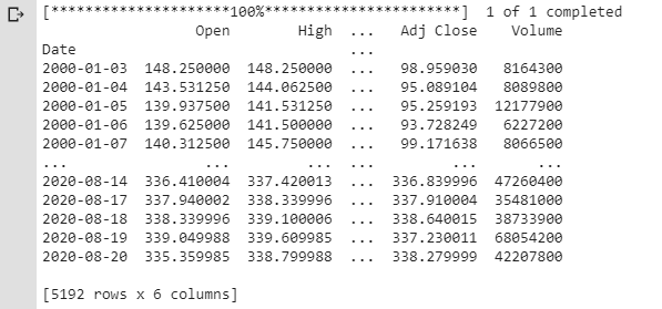
Next, we’re going to create a dataframe called df and download SPY data from 2000 to it.
#Here we're creating a dataframe for spy data from 2000-current
df = yf.download('spy',
  start='2000-01-01',
  end='2020-08-21',
  progress=True)
  #dauto_adjust=True,
  #actions='inline',) #adjust for stock splits and dividends
#print the dataframe to see what lives in it
print(df)
Finally, we’ll print the result of df so you can get an idea of what is inside of it.
We’re going to drop all the columns except Adj Close. Then we’ll rename it adj_close. Next, we’ll create a column labeled simple_rtn. This is the daily simple return or percent increase/decrease. The next line of code creates a logarithmic increase/decrease. Logarithmic gives equal bearing to the Y-axis and can be defined as follows, “A logarithmic price scale uses the percentage of change to plot data points, so, the scale prices are not positioned equidistantly. A linear price scale uses an equal value between price scales providing an equal distance between values.”
#only keep adj close
df = df.loc[:, ['Adj Close']]
df.rename(columns={'Adj Close':'adj_close'}, inplace=True)
#create column simple return
df['simple_rtn'] = df.adj_close.pct_change()
#create column logrithmic returns
df['log_rtn'] = np.log(df.adj_close/df.adj_close.shift(1))
print(df)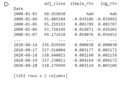
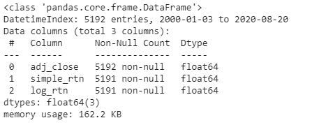
This next command just analyzes the data so you can spot-check what you’ve created.
#here we can analyze our data
df.info()
This next section describes what the daily increase/decrease of the SPY looks like. You can see statistically relevant information about S&P here.
#get statistical data on the data frame
df.describe()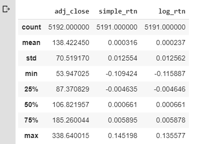
Next, we can see a distribution of adjustable close, logarithmic return, and simple return.
#view chart of data to get an overview of what lives in the data
import matplotlib.pyplot as plt
df.hist(bins=50, figsize=(20,15))
plt.show()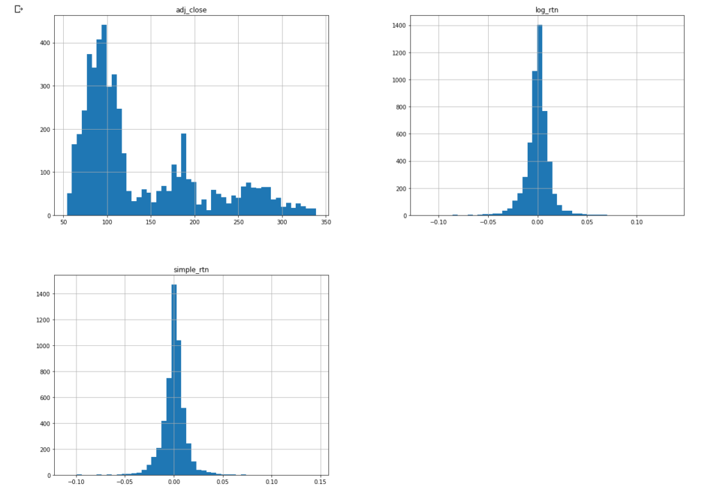
This is all for data normalization. You can now apply different algorithmic analyses to the data.